Fitting Baselines to Spectra

Tutorial Explaining hyperSpec’s Baseline Fitting Functions

Claudia Beleites^1,2,3,4,5, Vilmantas Gegzna

DIA Raman Spectroscopy Group, University of Trieste/Italy (2005–2008)
Spectroscopy $\cdot$ Imaging, IPHT, Jena/Germany (2008–2017)
ÖPV, JKI, Berlin/Germany (2017–2019)
Arbeitskreis Lebensmittelmikrobiologie und Biotechnologie, Hamburg University, Hamburg/Germany (2019 – 2020)
Chemometric Consulting and Chemometrix GmbH, Wölfersheim/Germany (since 2016)

2024-03-07

Source: vignettes/baseline.Rmd

baseline.Rmd

1 Introduction

This document discusses baseline correction methods that can be used with package hyperSpec. Package hyperSpec provides two fitting functions for polynomial baselines, spc_fit_poly() and spc_fit_poly_below(). Another possibility is spc_rubberband(), a “rubberband” method that determines support points by finding the convex hull of each spectrum. The baselines are then piecewise linear or (smoothing) splines through the support points.

Please note that a specialized package for baseline fitting, package baseline[1,2], exists that provides many more methods to fit baselines to spectroscopic data. Using package baseline with hyperSpec objects is demonstrated in vignette ("hyperspec").

2 Polynomial Baselines

In contrast to many other programs that provide baseline correction methods, package hyperSpec’s polynomial baseline functions do least squares fits. However, the baselines can be forced through particular points, if this behaviour is needed.

The main difference between the two functions is that spc_fit_poly() returns a least squares fit through the complete spectrum that is given in fit.to whereas spc_fit_poly_below() tries to find appropriate spectral regions to fit the baseline to.

2.1 Syntax and Parameters

spc_fit_poly(fit.to, apply.to = fit.to, poly.order = 1)

spc_fit_poly_below(fit.to, apply.to = fit.to, poly.order = 1, npts.min = NULL, noise = 0)

fit.to: hyperSpec object with the spectra whose baselines are to be fitted.
apply.to: hyperSpec object giving the spectral range, on which the baselines should be evaluated. If apply() is NULL, a hyperSpec object with the polynomial coefficients is returned instead of evaluated baselines.
poly.order: polynomial order of the baselines.
npts.min: minimal number of data points per spectrum to be used for the fit. Argument npts.min defaults to the larger of 3 times (poly.order + 1) or $\frac{1}{20th}$ of the number of data points per spectrum. If npts.min $\leq$ poly.order, a warning is issued and npts.min <- poly.order + 1 is used.
noise: a vector giving the amount of noise, see below.

2.2 General Use

Both functions fit the polynomial to the spectral range given in hyperSpec object fit.to. If apply.to is not NULL, the polynomials are evaluated on the spectral range of apply.to. Otherwise, the polynomial coefficients are returned.

Subtracting the baseline is up to the user, it is easily done as hyperSpec provides the - (minus) operator.

2.3 Fitting Polynomial Baselines Using Least Squares

Commonly, baselines are fit using (single) support points that are specified by the user. Also, usually $n + 1$ support point is used for a polynomial of order $n$. This approach is appropriate for spectra with high signal to noise ratio.

Such a baseline can be obtained by restricting the spectra in fit.to to the respective points (see figure 2.1):

# Load Raman spectra
file <- system.file("extdata/chondro_mini.rds", package = "hyperSpec")
chondro_mini <- readRDS(file)

bl <- spc_fit_poly(chondro_mini[, , c(633, 1788)], chondro_mini)

plot(chondro_mini, plot.args = list(ylim = c(200, 600)), col = 1:2)
plot(chondro_mini[, , c(633, 1788)],
  add = TRUE, col = 1:2,
  lines.args = list(type = "p", pch = 20)
)
plot(bl, add = TRUE, col = 1:2)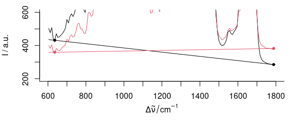

Fitting a linear baseline through two points.
If the signal to noise ratio is not ideal, wavelengths that work fine for one spectrum (black) may not be appropriate for another (red).

Figure 2.1: Fitting a linear baseline through two points. If the signal to noise ratio is not ideal, wavelengths that work fine for one spectrum (black) may not be appropriate for another (red).

However, if the signal to noise ratio is not ideal, a polynomial with $n + 1$ supporting points (i.e. with zero degrees of freedom) is subject to a considerable amount of noise. If on the other hand, more data points consisting of baseline only are available, the uncertainty on the polynomial can be reduced by a least squares fit.

Both spc_fit_poly() and spc_fit_poly_below() therefore provide least squares fitting for the polynomial.

Function spc_fit_poly() fits to the whole spectral region of fit.to. Thus, for baseline fitting the spectra need to be cut to appropriate wavelength ranges that do not contain any signal.

In order to speed up calculations, the least squares fit is done by using the Vandermonde matrix and solving the equation system by qr.solve().

This fit is not weighted. A spectral region with many data points therefore has greater influence on the resulting baseline than a region with just a few data points. It is up to the user to decide whether this should be corrected for by selecting appropriate numbers of data points (e.g. by using replicates of the shorter spectral region).

2.4 The Mechanism of Automatically Fitting the Baseline in `spc_fit_poly_below()`

Function spc_fit_poly_below() tries to automatically find appropriate spectral regions for baseline fitting. This is done by excluding spectral regions that contain signals from the baseline fitting. The idea is that all data points that lie above a fitted polynomial (initially through the whole spectrum, then through the remaining parts of the spectrum) will be treated as signal and thus be excluded from the baseline fitting.

The supporting points for the baseline polynomials are calculated iteratively:

A polynomial of the requested order is fit to the considered spectral range, initially to the whole spectrum given in fit.to
Only the parts of the spectrum that lie below this polynomial plus the noise are retained as supporting points for the next iteration.

These two steps are repeated until either:

no further points are excluded, or
the next polynomial would have less than npts.min supporting points.

The baselines and respective supporting points for each iteration of spc_fit_poly_below(chondro_mini[1], poly.order = 1) are shown in figure 2.2.

bl <- spc_fit_poly_below(chondro_mini[1], poly.order = 1, max.iter = 8, npts.min = 2, debuglevel = 3L)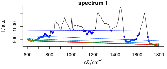

Figure 2.2: Iterative fitting of the baseline. The dots give the supporting points for the next iteration’s baseline, color: iterations.

2.5 Specifying the Spectral Range

plot(chondro_mini[1, , 1700 ~ 1750],
  lines.args = list(type = "b"),
  plot.args = list(ylim = range(chondro_mini[1, , 1700 ~ 1750]) + c(-50, 0))
)

bl <- spc_fit_poly_below(chondro_mini[1, , 1700 ~ 1750], NULL, poly.order = 1)
abline(bl[[]], col = "black")

plot(
  chondro_mini[1, , 1720 ~ 1750],
  lines.args = list(type = "p", pch = 19, cex = .6),
  col = "blue",
  add = T
)

bl <- spc_fit_poly_below(chondro_mini[1, , 1720 ~ 1750], NULL, poly.order = 1)
abline(bl[[]], col = "blue")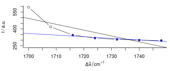

$Influence of `fit.to`{.r} on the baseline polynomial. The black baseline is fit to the spectral range 1700 - 1750 $cm^{-1}$, the blue to 1720 - 1750 $cm^{-1}$ only.$

Figure 2.3: Influence of fit.to on the baseline polynomial. The black baseline is fit to the spectral range 1700 - 1750 $cm^{-1}$, the blue to 1720 - 1750 $cm^{-1}$ only.

It is possible to exclude spectral regions that do not contribute to the baseline from the fitting, while the baseline is used for the whole spectrum. This selection of appropriate spectral regions is essential for spc_fit_poly(). But also spc_fit_poly_below() can benefit from narrower spectral ranges: the fitting gains speed. The default value for npts.min depends on the number of data points per spectrum. Thus one should also consider requiring more support points than the default value suggests.

system.time(spc_fit_poly_below(chondro_mini, NULL, npts.min = 20))
#>    user  system elapsed 
#>   0.002   0.000   0.003
system.time(spc_fit_poly_below(chondro_mini[, , c(min ~ 700, 1700 ~ max)], NULL, npts.min = 20))
#>    user  system elapsed 
#>   0.003   0.000   0.003

The choice of the spectral range in fit.to influences the resulting baselines to a certain extent, as becomes clear from figure 2.3.

2.6 Fitting Polynomials of Different Orders

bl <- spc_fit_poly_below(chondro_mini[1], poly.order = 0, debuglevel = 2, max.iter = 5)
#> Fitting with npts.min = 8
#> start: 150 support points
#> spectrum      1:    10 support points, noise = 0.0,   5 iterations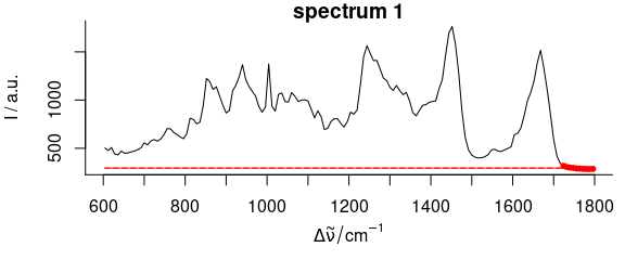

Baseline polynomial fit to the first spectrum of the chondro_mini data set of order 0 -- 2 (left to right).
The dots indicate the points used for the fitting of the polynomial.

Figure 2.4: Baseline polynomial fit to the first spectrum of the chondro_mini data set of order 0 – 2 (left to right). The dots indicate the points used for the fitting of the polynomial.

bl <- spc_fit_poly_below(chondro_mini[1], poly.order = 1, debuglevel = 2, max.iter = 5)
#> Fitting with npts.min = 8
#> start: 150 support points
#> Warning in spc_fit_poly_below(chondro_mini[1], poly.order = 1, debuglevel = 2, : Stopped after 5
#> iterations with 14 support points.
#> spectrum      1:    14 support points, noise = 0.0,   5 iterations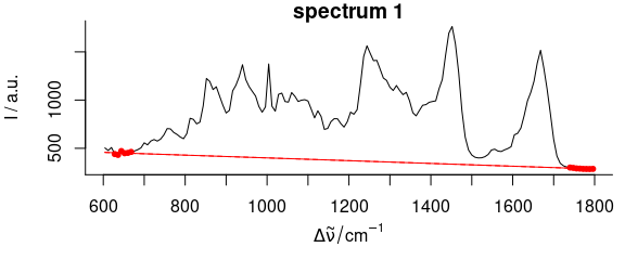

Figure 2.5: Baseline polynomial fit to the first spectrum of the chondro_mini data set of order 0 – 2 (left to right). The dots indicate the points used for the fitting of the polynomial.

bl <- spc_fit_poly_below(chondro_mini[1], poly.order = 2, debuglevel = 2, max.iter = 5)
#> Fitting with npts.min = 9
#> start: 150 support points
#> spectrum      1:    11 support points, noise = 0.0,   5 iterations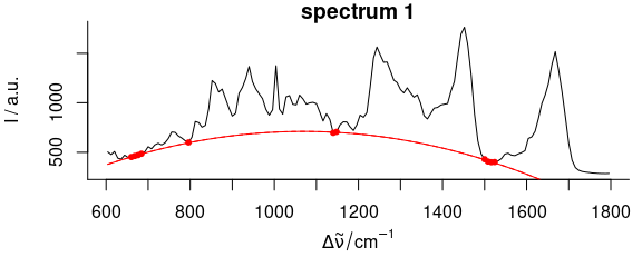

Figure 2.6: Baseline polynomial fit to the first spectrum of the chondro_mini data set of order 0 – 2 (left to right). The dots indicate the points used for the fitting of the polynomial.

Figures 2.4, 2.5, 2.6 show the resulting baseline polynomial of spc_fit_poly_below (chondro_mini [1], poly.order = order) with order $=$ 0 to 3 for the first spectrum of the chondro_mini data set.

2.7 The Noise Level

spc <- new("hyperSpec", spc = matrix(rnorm(100, mean = 100, sd = 2), ncol = 100))
noise <- 4
spc_fit_poly_below(spc, poly.order = 0, noise = noise, debuglevel = 2)
#> hyperSpec object
#>    1 spectra
#>    1 data columns
#>    100 data points / spectrum
plot(spc_fit_poly_below(spc, poly.order = 0), col = "black", add = T)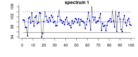

Iterative fitting of the baseline with noise level.
Effects of the noise parameter on the baseline of a spectrum consisting only of noise and offset: without giving `noise`{.r} the resulting baseline (black) is clearly too low.
A noise level of 4 results in the blue baseline.

Figure 2.7: Iterative fitting of the baseline with noise level. Effects of the noise parameter on the baseline of a spectrum consisting only of noise and offset: without giving noise the resulting baseline (black) is clearly too low. A noise level of 4 results in the blue baseline.

bl <- spc_fit_poly_below(chondro_mini[1], poly.order = 1, noise = 15, max.iter = 8, debuglevel = 3L)
#> Warning in spc_fit_poly_below(chondro_mini[1], poly.order = 1, noise = 15, : Stopped after 8
#> iterations with 13 support points.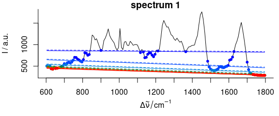

Iterative fitting of the baseline with noise level.
The baseline fitting with noise level on the complete spectrum.
Colour: iterations, dots: supporting points for the respectively next baseline.
Dashed: baseline plus noise.
All points above this line are excluded from the next iteration.

Figure 2.8: Iterative fitting of the baseline with noise level. The baseline fitting with noise level on the complete spectrum. Colour: iterations, dots: supporting points for the respectively next baseline. Dashed: baseline plus noise. All points above this line are excluded from the next iteration.

Besides defining a minimal number of supporting points, a “noise level” may be given. Consider a spectral range consisting only of noise. The upper part of figures 2.7, 2.8 illustrate the problem. As the baseline fitting algorithm cannot distinguish between noise and real bands appearing above the fitted polynomial, the resulting baseline (black) is too low if the noise parameter is not given.

Setting the noise level to 4 (2 standard deviations), the fitting converges immediately with a much better result. The resulting baselines for spc_fit_poly_below (chondro_mini [1], poly.order = 1, noise = 12) of the whole spectrum are shown in the middle and lower part of figure 2.8.

The noise may be a single value for all spectra, or a vector with the noise level for each of the spectra separately.

3 Rubberband Method

Particularly Raman spectra often show increasing background towards $\Delta\tilde\nu = 0$. In this case, polynomial baselines often either need high order or residual background is left in the spectra.

In that case, smoothing splines fitted through the supporting points are a good alternative.

For the paracetamol spectrum (fig. 3.1, 3.2), a noise level of 300 counts and the equivalent of 20 degrees of freedom work well.

bl <- spc_rubberband(paracetamol[, , 175 ~ 1800], noise = 300, df = 20)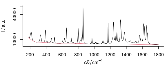

plot(paracetamol[, , 175 ~ 1800])
plot(bl, add = TRUE, col = 2)

Rubberband baselines for the paracetamol spectrum:`paracetamol`{.r} with the `rubberband()`{.r} fitted baseline.

Figure 3.1: Rubberband baselines for the paracetamol spectrum:paracetamol with the rubberband() fitted baseline.

plot(paracetamol[, , 175 ~ 1800] - bl)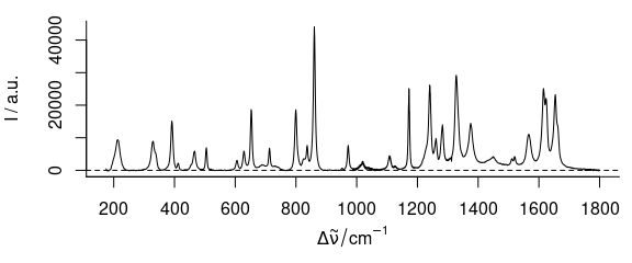

Figure 3.2: Rubberband baselines for the paracetamol spectrum: corrected spectrum.

However, there is possibly some background left between 1200 and 1750 cm^-1 where the original spectrum is slightly concave. This can be corrected by bending the spectrum before applying the rubberband correction (fig. 3.3, 3.4):

bend <- 5e4 * wl_eval(paracetamol[, , 175 ~ 1800], function(x) x^2, normalize.wl = normalize_01)
bl <- spc_rubberband(paracetamol[, , 175 ~ 1800] + bend) - bend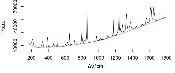

plot(paracetamol[, , 175 ~ 1800] + bend)
plot(bl + bend, add = T, col = 2)

Rubberband baselines for the paracetamol spectrum after bending: bent `paracetamol`{.r} spectrum and rubberband baseline.

Figure 3.3: Rubberband baselines for the paracetamol spectrum after bending: bent paracetamol spectrum and rubberband baseline.

plot(paracetamol[, , 175 ~ 1800] - bl)

Figure 3.4: Rubberband baselines for the paracetamol spectrum after bendin: corrected spectrum.

Session Info

sessioninfo::session_info("hyperSpec")
#> ─ Session info ───────────────────────────────────────────────────────────────────────────────────
#>  setting  value
#>  version  R version 4.3.3 (2024-02-29)
#>  os       Ubuntu 22.04.4 LTS
#>  system   x86_64, linux-gnu
#>  ui       X11
#>  language en
#>  collate  C.UTF-8
#>  ctype    C.UTF-8
#>  tz       UTC
#>  date     2024-03-07
#>  pandoc   3.1.11 @ /opt/hostedtoolcache/pandoc/3.1.11/x64/ (via rmarkdown)
#> 
#> ─ Packages ───────────────────────────────────────────────────────────────────────────────────────
#>  ! package        * version      date (UTC) lib source
#>    brio             1.1.4        2023-12-10 [2] RSPM
#>    callr            3.7.5        2024-02-19 [2] RSPM
#>    cli              3.6.2        2023-12-11 [2] RSPM
#>    colorspace       2.1-0        2023-01-23 [2] RSPM
#>    crayon           1.5.2        2022-09-29 [2] RSPM
#>    deldir           2.0-4        2024-02-28 [2] RSPM
#>    desc             1.4.3        2023-12-10 [2] RSPM
#>    diffobj          0.3.5        2021-10-05 [2] RSPM
#>    digest           0.6.34       2024-01-11 [2] RSPM
#>    dplyr            1.1.4        2023-11-17 [2] RSPM
#>    evaluate         0.23         2023-11-01 [2] RSPM
#>    fansi            1.0.6        2023-12-08 [2] RSPM
#>    farver           2.1.1        2022-07-06 [2] RSPM
#>    fs               1.6.3        2023-07-20 [2] RSPM
#>    generics         0.1.3        2022-07-05 [2] RSPM
#>    ggplot2        * 3.5.0        2024-02-23 [2] RSPM
#>    glue             1.7.0        2024-01-09 [2] RSPM
#>    gtable           0.3.4        2023-08-21 [2] RSPM
#>    hyperSpec      * 0.200.0.9000 2024-03-07 [1] local
#>    hySpc.testthat   0.2.1        2020-06-24 [2] RSPM
#>    interp           1.1-6        2024-01-26 [2] RSPM
#>    isoband          0.2.7        2022-12-20 [2] RSPM
#>    jpeg             0.1-10       2022-11-29 [2] RSPM
#>    jsonlite         1.8.8        2023-12-04 [2] RSPM
#>    labeling         0.4.3        2023-08-29 [2] RSPM
#>    lattice        * 0.22-5       2023-10-24 [4] CRAN (R 4.3.3)
#>    latticeExtra     0.6-30       2022-07-04 [2] RSPM
#>    lazyeval         0.2.2        2019-03-15 [2] RSPM
#>    lifecycle        1.0.4        2023-11-07 [2] RSPM
#>    magrittr         2.0.3        2022-03-30 [2] RSPM
#>    MASS             7.3-60.0.1   2024-01-13 [4] CRAN (R 4.3.3)
#>    Matrix           1.6-5        2024-01-11 [4] CRAN (R 4.3.3)
#>    mgcv             1.9-1        2023-12-21 [4] CRAN (R 4.3.3)
#>    munsell          0.5.0        2018-06-12 [2] RSPM
#>    nlme             3.1-164      2023-11-27 [4] CRAN (R 4.3.3)
#>    pillar           1.9.0        2023-03-22 [2] RSPM
#>    pkgbuild         1.4.3        2023-12-10 [2] RSPM
#>    pkgconfig        2.0.3        2019-09-22 [2] RSPM
#>    pkgload          1.3.4        2024-01-16 [2] RSPM
#>    png              0.1-8        2022-11-29 [2] RSPM
#>    praise           1.0.0        2015-08-11 [2] RSPM
#>    processx         3.8.3        2023-12-10 [2] RSPM
#>    ps               1.7.6        2024-01-18 [2] RSPM
#>    R6               2.5.1        2021-08-19 [2] RSPM
#>    RColorBrewer     1.1-3        2022-04-03 [2] RSPM
#>    Rcpp             1.0.12       2024-01-09 [2] RSPM
#>  R RcppEigen        <NA>         <NA>       [?] <NA>
#>    rematch2         2.1.2        2020-05-01 [2] RSPM
#>    rlang            1.1.3        2024-01-10 [2] RSPM
#>    rprojroot        2.0.4        2023-11-05 [2] RSPM
#>    scales           1.3.0        2023-11-28 [2] RSPM
#>    testthat         3.2.1        2023-12-02 [2] RSPM
#>    tibble           3.2.1        2023-03-20 [2] RSPM
#>    tidyselect       1.2.0        2022-10-10 [2] RSPM
#>    utf8             1.2.4        2023-10-22 [2] RSPM
#>    vctrs            0.6.5        2023-12-01 [2] RSPM
#>    viridisLite      0.4.2        2023-05-02 [2] RSPM
#>    waldo            0.5.2        2023-11-02 [2] RSPM
#>    withr            3.0.0        2024-01-16 [2] RSPM
#>    xml2             1.3.6        2023-12-04 [2] RSPM
#> 
#>  [1] /tmp/RtmpwJcUHX/temp_libpath18f414eab874
#>  [2] /home/runner/work/_temp/Library
#>  [3] /opt/R/4.3.3/lib/R/site-library
#>  [4] /opt/R/4.3.3/lib/R/library
#> 
#>  R ── Package was removed from disk.
#> 
#> ──────────────────────────────────────────────────────────────────────────────────────────────────

References

[1]

K.H. Liland, B.-H. Mevik, Baseline: Baseline correction of spectra, 2023. https://github.com/khliland/baseline/.

[2]

K.H. Liland, T. Almøy, B.-H. Mevik, Optimal choice of baseline correction for multivariate calibration of spectra, Applied Spectroscopy. 64 (2010) 1007–1016. https://doi.org/10.1366/000370210792434350.