Raman Spectra of Chondrocytes in Cartilage

Example Workflow for 2D Raman Spectra Dataset `chondro`

Claudia Beleites^1,2,3,4,5, Vilmantas Gegzna

DIA Raman Spectroscopy Group, University of Trieste/Italy (2005–2008)
Spectroscopy $\cdot$ Imaging, IPHT, Jena/Germany (2008–2017)
ÖPV, JKI, Berlin/Germany (2017–2019)
Arbeitskreis Lebensmittelmikrobiologie und Biotechnologie, Hamburg University, Hamburg/Germany (2019 – 2020)
Chemometric Consulting and Chemometrix GmbH, Wölfersheim/Germany (since 2016)

2023-04-23

Source: vignettes/hySpc-chondro.Rmd

hySpc-chondro.Rmd

1 Introduction

This vignette describes the chondro data set. It shows a complete data analysis work flow on a Raman map demonstrating frequently needed preprocessing methods:

baseline correction,
normalization,
smoothing / interpolating spectra,
preprocessing the spatial grid,

as well as other basic work techniques:

plotting spectra,
plotting false color maps,
cutting the spectral range,
selecting (extracting) or deleting spectra, and
aggregating spectra (e.g., calculating cluster mean spectra).

The chemometric methods used are:

Principal Component Analysis (PCA) and
Hierarchical Cluster Analysis,

showing how to use data analysis procedures provided by R and other packages.

2 The Data Set

Raman spectra of a cartilage section were measured on each point of a grid, resulting in a so-called Raman map. Figure 2.1 shows a microscope picture of the measured area and its surroundings.

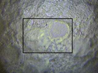
$Microphotograph of the cartilage section. The frame indicates the measurement area of $35×25 \mu m.$$

Figure 2.1: Microphotograph of the cartilage section. The frame indicates the measurement area of $35×25 \mu m.$

The measurement parameters were:

Excitation wavelength: 633 nm
Exposure time: 10 s per spectrum
Objective: 100×, NA 0.85
Measurement grid: 35 × 25 $\mu m$, 1 $\mu m$ step size
Spectrometer: Renishaw InVia

3 Data Import

Renishaw provides a converter to export their proprietary data in a so-called long format ASCII file. Raman maps are exported having four columns, y, x, raman shift, and intensity. Package hySpc.read.txt comes with a function to import such files, hySpc.read.txt::read_txt_Renishaw(). The function assumes a map as default, but can also handle single spectra (data = "spc"), time series (data = "ts"), and depth profiles (data = "depth"). In addition, large files may be processed in chunks. In order to speed up the reading read_txt_Renishaw() does not allow missing values, but it does work with NA.

# Download file from:
raw_data_url <-
  "https://media.githubusercontent.com/media/cbeleites/hyperSpec/master/Vignettes/fileio/txt.Renishaw/chondro.gz"
dir.create("rawdata", showWarnings = FALSE)
download.file(raw_data_url, "rawdata/chondro.gz")

# Read the raw data and make a hyperSpec object
chondro <- hySpc.read.txt::read_txt_Renishaw("rawdata/chondro.gz", data = "xyspc")
chondro
#> hyperSpec object
#>    875 spectra
#>    4 data columns
#>    1272 data points / spectrum

To get an overview of the spectra (figure 3.1):

plot(chondro, "spcprctl5")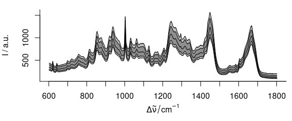

Figure 3.1: The raw spectra: median, 16^th and 84^th, and 5^th and 95^th percentile spectra.

A mean intensity map (figure 3.2) is produced by:

# Set a color palette
seq_palette <- colorRampPalette(c("white", "dark green"), space = "Lab")

plotmap(chondro, func.args = list(na.rm = TRUE), col.regions = seq_palette(20))
#> Warning: Function 'plotmap' is deprecated. 
#> Use function 'plot_map' instead.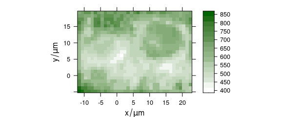

Figure 3.2: The sum intensity of the raw spectra.

Function plotmap() squeezes all spectral intensities into a summary characteristic for the whole spectrum. This function defaults to the mean(). Further arguments that should be handed to this function can be given in list func.args. As the raw data contains NAs due to deleting cosmic ray spikes, this argument is needed here.

4 Preprocessing

As usual in Raman spectroscopy of biological tissues, the spectra need some preprocessing.

4.1 Aligning the Spatial Grid

The spectra were acquired on a regular square grid of measurement positions over the sample. The hyperSpec object, however, does not store the data on this grid but rather stores the position where the spectra were taken. This allows more handling of irregular point patterns, and of sparse measurements where not a complete (square) is retained but only few positions on this grid.

Occasionally, numeric or rounding errors will lead to seemingly irregular spacing of the data points. This is most obvious in false-colour maps of the sample (fig. 3.2, as plotmap by default uses panel.levelplot.raster, which assumes a regular grid is underlying the data. The symptoms are warnings “'x' values are not equispaced; output may be wrong” and white stripes in the false colour map (fig. 4.1), which occur even thought the points are almost at their correct place (fig. 4.2).

## disturb a few points
chondro$x[500] <- chondro$x[500] + rnorm(1, sd = 0.01)
chondro$y[660] <- chondro$y[660] + rnorm(1, sd = 0.01)

plotmap(chondro, col.regions = seq_palette(20))
#> Warning: Function 'plotmap' is deprecated. 
#> Use function 'plot_map' instead.
#> Warning in (function (x, y, z, subscripts, at = pretty(z), ..., col.regions = regions$col, : 'x'
#> values are not equispaced; output may be wrong
#> Warning in (function (x, y, z, subscripts, at = pretty(z), ..., col.regions = regions$col, : 'y'
#> values are not equispaced; output may be wrong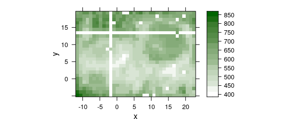

Figure 4.1: Rounding erros in the point coordinates of lateral measurement grid: (A) off-grid points cause stripes.

library("latticeExtra")
plotmap(chondro,
  col.regions = seq_palette(20), panel = panel.levelplot.points,
  col = NA, pch = 22, cex = 1.9
)
#> Warning: Function 'plotmap' is deprecated. 
#> Use function 'plot_map' instead.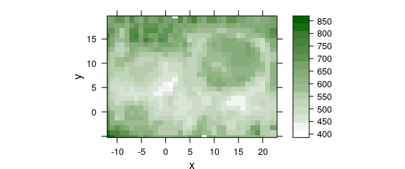

Figure 4.2: Rounding erros in the point coordinates of lateral measurement grid: (B) slightly wrong coordinages.

Such slight rounding errors can be corrected by raster_fit() or raster_make(). Function raster_fit() needs the step size of the raster and a starting coordinate, whereas raster_make() tries to guess these parameters for raster_fit(). As long as just a few points are affected by rounding errors, raster_make() works fine:

chondro$x <- raster_fit(chondro$x)$x
chondro$y <- raster_fit(chondro$y)$x

the result is shown in figure 4.3.

plotmap(chondro, col.regions = seq_palette(20))
#> Warning: Function 'plotmap' is deprecated. 
#> Use function 'plot_map' instead.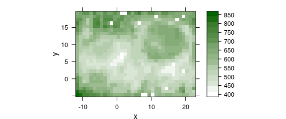

Figure 4.3: Rounding erros in the point coordinates of lateral measurement grid: (C) corrected grid.

Rounding erros in the point coordinates of lateral measurement grid.
**(A)** Off-grid points cause stripes.
**(B)** Slightly wrong coordinages.
**(C)** Corrected grid.

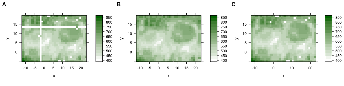
Figure 4.4: Rounding erros in the point coordinates of lateral measurement grid. (A) Off-grid points cause stripes. (B) Slightly wrong coordinages. (C) Corrected grid.

4.2 Spectral Smoothing

As the overview shows that the spectra contain NAs (from cosmic spike removal that was done previously), the first step is to remove these. Also, the wavelength axis of the raw spectra is not evenly spaced (the data points are between 0.85 and 1 $cm^{-1}$ apart from each other). Furthermore, it would be good to trade some spectral resolution for higher signal to noise ratio. All three of these issues are tackled by interpolating and smoothing of the wavelength axis by spc_loess(). The resolution is to be reduced to 8 $cm^{-1}$, or 4 $cm^{-1}$ data point spacing.

chondro <- spc_loess(chondro, seq(602, 1800, 4))
chondro
#> hyperSpec object
#>    875 spectra
#>    4 data columns
#>    300 data points / spectrum

The spectra are now the same as in the data set chondro. However, the data set also contains the clustering results (see at the very end of this document). They are stored for saving as the distributed demo data:

spectra_to_save <- chondro

4.3 Baseline Correction

The next step is a linear baseline correction. spc_fit_poly_below() tries to automatically find appropriate support points for polynomial baselines. The default is a linear baseline, which is appropriate in our case:

baselines <- spc_fit_poly_below(chondro)
chondro <- chondro - baselines

4.4 Normalization

As the spectra are quite similar, area normalization should work well:

chondro <- chondro / rowMeans(chondro)
plot(chondro, "spcprctl5")

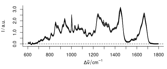
Figure 4.5: The spectra after smoothing, baseline correction, and normalization.

Note that normalization effectively cancels the information of one variate (wavelength), it introduces a collinearity. If needed, this collinearity can be broken by removing one of the variates involved in the normalization. Note that the chondro object shipped with package hyperSpec set has multiple collinearities as only the first 10 principal components are shipped (see below).

For the results of these preprocessing steps, see figure 4.5.

4.5 Subtracting the Overall Composition

The spectra are very homogeneous, but I’m interested in the differences between the different regions of the sample. Subtracting the minimum spectrum cancels out the matrix composition that is common to all spectra. But the minimum spectrum also picks up a lot of noise. So instead, the 5^th percentile spectrum is subtracted:

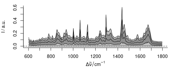
chondro <- chondro - quantile(chondro, 0.05)
plot(chondro, "spcprctl5")

Figure 4.6: The spectra after subtracting the 5^th percentile spectrum.

The resulting data set is shown in figure 4.6. Some interesting differences start to show up: there are distinct lipid bands in some but not all of the spectra.

4.6 Outlier Removal by Principal Component Analysis (PCA)

PCA is a technique that decomposes the data into scores and loadings (virtual spectra). It is known to be quite sensitive to outliers. Thus, I use it for outlier detection. The resulting scores and loadings are put again into hyperSpec objects by decomposition():

pca <- prcomp(chondro, center = TRUE)

scores <- decomposition(chondro, pca$x,
  label.wavelength = "PC",
  label.spc = "score / a.u."
)

loadings <- decomposition(chondro, t(pca$rotation),
  scores = FALSE,
  label.spc = "loading I / a.u."
)

Plotting the scores of each PC against all other gives a good idea where to look for outliers.

pairs(scores[[, , 1:7]], pch = 19, cex = 0.5)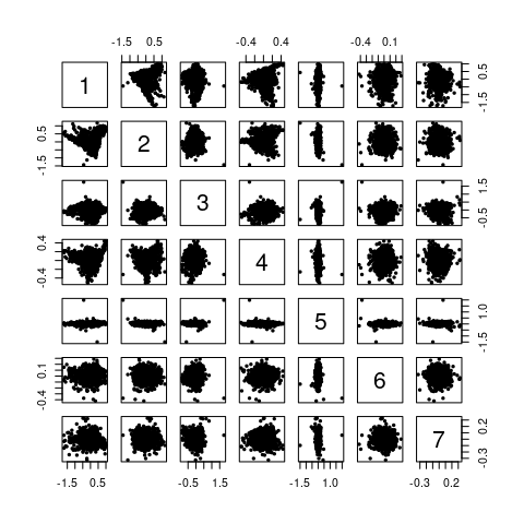

The `pairs()`{.r} plot of the first 7 scores.

Figure 4.7: The pairs() plot of the first 7 scores.

Now the spectra can be found either by plotting two scores against each other (by plot()) and identifying with identify(), or they can be identified in the score map by map.identify(). There is also a function to identify spectra in a spectra plot, identify_spc(), which could be used to identify principal components that are heavily influenced, e.g., by cosmic ray spikes.

## omit the first 4 PCs
out <- map.identify(scores[, , 5])
out <- c(out, map.identify(scores[, , 6]))
out <- c(out, map.identify(scores[, , 7]))

out
#> [1] 105 140 216 289  75  69
outcols <- c("red", "blue", "#800080", "orange", "magenta", "brown")

cols <- rep("black", nrow(chondro))
cols[out] <- outcols

We can check our findings by comparing the spectra to the bulk of spectra (figure 4.8):

plot(chondro[1],
  plot.args = list(ylim = c(1, length(out) + .7)),
  lines.args = list(type = "n")
)

for (i in seq(along = out)) {
  plot(chondro, "spcprctl5", yoffset = i, add = TRUE, col = "gray")
  plot(chondro[out[i]],
    yoffset = i, col = outcols[i], add = TRUE,
    lines.args = list(lwd = 2)
  )
  text(600, i + .33, out[i])
}

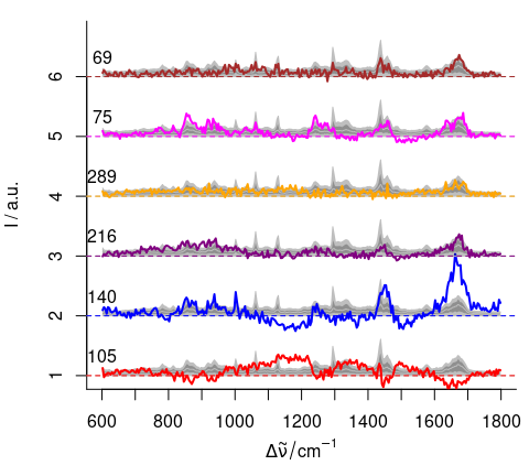
Figure 4.8: The suspected outlier spectra.

and also by looking where these spectra appear in the scores pairs() plot (figure 4.9):

pch <- rep(46L, nrow(chondro))
pch[out] <- 19L

pairs(scores[[, , 1:7]], pch = pch, cex = 1, col = cols)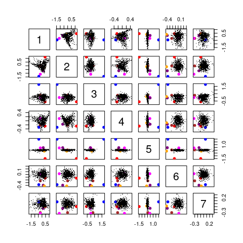

The `pairs()`{.r} plot of the first 7 scores with suspected outliers.

Figure 4.9: The pairs() plot of the first 7 scores with suspected outliers.

Finally, the outliers are removed:

chondro <- chondro[-out]

5 Hierarchical Cluster Analysis (HCA)

HCA merges objects according to their (dis)similarity into clusters. The result is a dendrogram, a graph stating at which level two objects are similar and thus grouped together.

The first step in HCA is the choice of the distance. The R function dist() offers a variety of distance measures to be computed. The so-called Pearson distance $D^2_{Pearson}=\frac{1-\mathrm{COR}\left(X\right)}{2}$ is popular in data analysis of vibrational spectra and is provided by package hyperSpec’s pearson.dist() function.

Also for computing the dendrogram, a number of choices are available. Here we choose Ward’s method, and, as it uses Euclidean distance for calculating the dendrogram, Euclidean distance also for the distance matrix:

dist <- dist(chondro)
dendrogram <- hclust(dist, method = "ward.D2")

plot(dendrogram, labels = FALSE)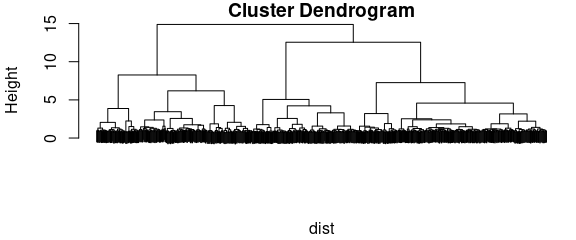

Figure 5.1: Dendogram.

In order to get clusters, the dendrogram is cut at a level specified either by height or by the number of clusters.

chondro$clusters <- as.factor(cutree(dendrogram, k = 3))
cols <- c("dark blue", "orange", "#C02020")

The result for $k$ = 3 clusters is plotted as a map (figure 5.2). If the color-coded variate (left hand side of the formula) is a factor, the legend bar does not show intermediate colors, and hyperSpec’s levelplot() method uses the levels of the factor for the legend.

Thus meaningful names are assigned

levels(chondro$clusters) <- c("matrix", "lacuna", "cell")

and the cluster membership map is plotted:

print(plotmap(chondro, clusters ~ x * y, col.regions = cols))
#> Warning: Function 'plotmap' is deprecated. 
#> Use function 'plot_map' instead.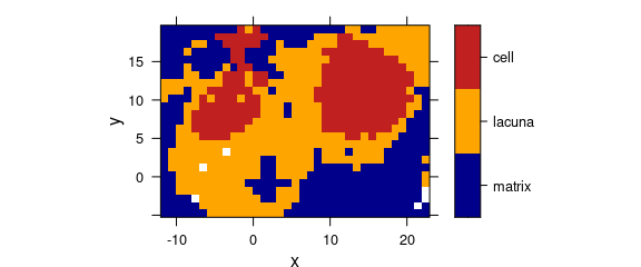

Figure 5.2: Hierarchical cluster analysis: the cluster map for $k=3$ clusters.

The cluster membership can also be marked in the dendrogram:

par(xpd = TRUE) # allow plotting the markers into the margin
plot(dendrogram, labels = FALSE, hang = -1)
mark_groups_in_dendrogram(dendrogram, chondro$clusters, col = cols)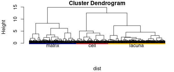

Figure 5.3: Hierarchical cluster analysis: the dendrogram.

Figure 5.3 shows the dendrogram and 5.2 the resulting cluster map. The three clusters correspond to the cartilage matrix, the lacuna and the cells. The left cell is destroyed and its contents are leaking into the matrix, while the right cells looks intact.

We can plot the cluster mean spectra $\pm$ 1 standard deviation using aggregate() (see figure 5.4):

cluster.means <- aggregate(chondro, chondro$clusters, mean_pm_sd)

op <- par(las = 1, mar = c(4, 6, 1, 1), mgp = c(4, 1, 0))
plot(cluster.means, stacked = ".aggregate", fill = ".aggregate", col = cols)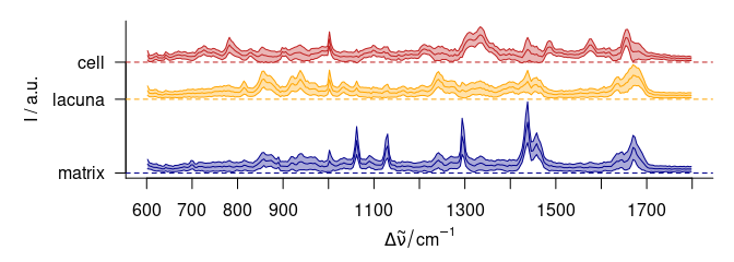

$The cluster mean $\pm$ 1 standard deviation spectra. The blue cluster shows distinct lipid bands, the yellow cluster collagen, and the red cluster proteins and nucleic acids.$

Figure 5.4: The cluster mean $\pm$ 1 standard deviation spectra. The blue cluster shows distinct lipid bands, the yellow cluster collagen, and the red cluster proteins and nucleic acids.

par(op)

6 Plotting a False-Colour Map of Certain Spectral Regions

Package hyperSpec comes with a sophisticated interface for specifying spectral ranges. Expressing things like 1000$cm^{-1}$ $\pm$ 1 data points is easily possible. Thus, we can have a fast look at the nucleic acid distribution, using the DNA bands at 728, 782, 1098, 1240, 1482, and 1577 $cm^{-1}:$

DNAcols <- colorRampPalette(c("white", "gold", "dark green"), space = "Lab")(20)
plotmap(chondro[, , c(728, 782, 1098, 1240, 1482, 1577)],
  col.regions = DNAcols
)
#> Warning: Function 'plotmap' is deprecated. 
#> Use function 'plot_map' instead.

Figure 6.1: False color map of DNA.

The result is shown in figure 6.1. While the nucleus of the right cell shows up nicely, only low concentration remainders are detected of the left cell.

7 Smoothed False-Colour Maps and Interpolation

As we plotted only a few selected wavelenths, figure 6.1 is quite noisy. Smoothing interpolation could help. In R, such a smoother is mostly seen as a model, whose predictions are then displayed as smooth map (fig. 7.1). This smoothing model can be calculated on the fly, e.g., by using the panel.2dsmoother() wrapper provided by package latticeExtra:

plotmap(chondro[, , c(728, 782, 1098, 1240, 1482, 1577)],
  col.regions = DNAcols,
  panel = panel.2dsmoother, args = list(span = 0.05)
)
#> Warning: Function 'plotmap' is deprecated. 
#> Use function 'plot_map' instead.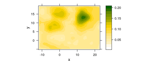

Figure 7.1: False colour map of the DNA band intensities: smoothed DNA abundance.

For interpolation (i.e., no smoothing at the available data points), a Voronoi plot (a.k.a. Delaunay triangulation) is basically a 2d constant interpolation: each point in space has the same z/color value as its closest available point. For a full rectangular grid, this corresponds to the usual square/rectangular pixel plot. With missing points, differences become clear (fig. 7.2):

tmp <- sample(chondro[, , c(728, 782, 1098, 1240, 1482, 1577)], 500)

plotmap(tmp, col.regions = DNAcols)
#> Warning: Function 'plotmap' is deprecated. 
#> Use function 'plot_map' instead.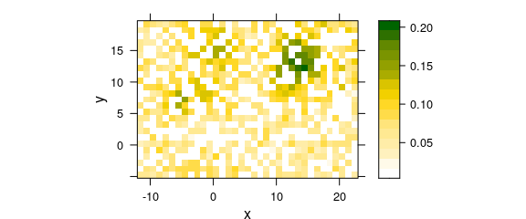

Figure 7.2: Two-dimesional (2D) “constant” interpolation with missing values: omitting missing data points.

plotmap(tmp,
  col.regions = DNAcols,
  panel = panel.voronoi, pch = 19, col = "black", cex = 0.1
)
#> Warning: Function 'plotmap' is deprecated. 
#> Use function 'plot_map' instead.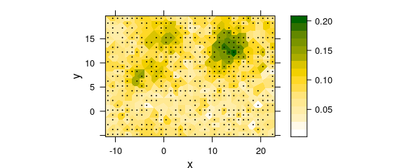

Figure 7.3: Two-dimesional (2D) “constant” interpolation with missing values: Delaunay triangulation / Voronoi plot.

The 2D linear interpolation can be done, e.g., by the functions provided by package package akima. However, they do not follow the model-predict paradigm, but instead do directly return an object suitable for base plotting with image() (fig. 7.4):

if (require("akima")) {
  tmp <- rowMeans(chondro[[, , c(728, 782, 1098, 1240, 1482, 1577)]])
  chondro.bilinear <- interp(chondro$x, chondro$y, as.numeric(tmp), nx = 100, ny = 100)

  image(chondro.bilinear,
    xlab = labels(chondro, "x"), ylab = labels(chondro, "y"),
    col = DNAcols
  )
} else {
  plot(NULL, xlim = c(0, 1), ylim = c(0, 1))
  text(0.5, 0.5, 'Package "akima" is required to create this plot')
}
#> Warning in interp(chondro$x, chondro$y, as.numeric(tmp), nx = 100, ny = 100): collinear points,
#> trying to add some jitter to avoid colinearities!
#> Warning in interp(chondro$x, chondro$y, as.numeric(tmp), nx = 100, ny = 100): success:
#> collinearities reduced through jitter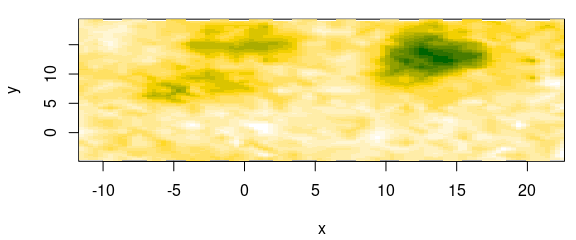

Figure 7.4: Two-dimensional (2D) interpolation.

8 Saving the data set

Finally, the example data set is put together and saved. In order to keep the package size small, only a PCA-compressed version with 10 PCs is shipped as example data set of the package.

spectra_to_save$clusters <- factor(NA, levels = levels(chondro$clusters))
spectra_to_save$clusters[-out] <- chondro$clusters

pca <- prcomp(spectra_to_save)

.chondro_scores <- pca$x[, seq_len(10)]
.chondro_loadings <- pca$rot[, seq_len(10)]
.chondro_center <- pca$center
.chondro_wl <- wl(chondro)
.chondro_labels <- lapply(labels(chondro), as.expression)
.chondro_extra <- spectra_to_save$..

chondro <- new("hyperSpec",
  spc = tcrossprod(.chondro_scores, .chondro_loadings) +
    rep(.chondro_center, each = nrow(.chondro_scores)),
  wavelength = .chondro_wl,
  data = .chondro_extra,
  labels = .chondro_labels
)

This is the file distributed with package hyperSpec as example data set.

Session Info

Session info

sessioninfo::session_info("hyperSpec")
#> ─ Session info ───────────────────────────────────────────────────────────────────────────────────
#>  setting  value
#>  version  R version 4.3.0 (2023-04-21)
#>  os       Ubuntu 22.04.2 LTS
#>  system   x86_64, linux-gnu
#>  ui       X11
#>  language en
#>  collate  C.UTF-8
#>  ctype    C.UTF-8
#>  tz       UTC
#>  date     2023-04-23
#>  pandoc   2.19.2 @ /usr/bin/ (via rmarkdown)
#> 
#> ─ Packages ───────────────────────────────────────────────────────────────────────────────────────
#>  package        * version      date (UTC) lib source
#>  brio             1.1.3        2021-11-30 [2] RSPM
#>  callr            3.7.3        2022-11-02 [2] RSPM
#>  cli              3.6.1        2023-03-23 [2] RSPM
#>  colorspace       2.1-0        2023-01-23 [2] RSPM
#>  crayon           1.5.2        2022-09-29 [2] RSPM
#>  deldir           1.0-6        2021-10-23 [2] RSPM
#>  desc             1.4.2        2022-09-08 [2] RSPM
#>  diffobj          0.3.5        2021-10-05 [2] RSPM
#>  digest           0.6.31       2022-12-11 [2] RSPM
#>  dplyr            1.1.2        2023-04-20 [2] RSPM
#>  ellipsis         0.3.2        2021-04-29 [2] RSPM
#>  evaluate         0.20         2023-01-17 [2] RSPM
#>  fansi            1.0.4        2023-01-22 [2] RSPM
#>  farver           2.1.1        2022-07-06 [2] RSPM
#>  fs               1.6.1        2023-02-06 [2] RSPM
#>  generics         0.1.3        2022-07-05 [2] RSPM
#>  ggplot2        * 3.4.2        2023-04-03 [2] RSPM
#>  glue             1.6.2        2022-02-24 [2] RSPM
#>  gtable           0.3.3        2023-03-21 [2] RSPM
#>  hyperSpec      * 0.200.0.9000 2023-04-23 [2] Custom
#>  hySpc.testthat   0.2.1.9000   2023-04-23 [2] Custom
#>  interp           1.1-4        2023-03-31 [2] RSPM
#>  isoband          0.2.7        2022-12-20 [2] RSPM
#>  jpeg             0.1-10       2022-11-29 [2] RSPM
#>  jsonlite         1.8.4        2022-12-06 [2] RSPM
#>  labeling         0.4.2        2020-10-20 [2] RSPM
#>  lattice        * 0.21-8       2023-04-05 [4] CRAN (R 4.3.0)
#>  latticeExtra   * 0.6-30       2022-07-04 [2] RSPM
#>  lazyeval         0.2.2        2019-03-15 [2] RSPM
#>  lifecycle        1.0.3        2022-10-07 [2] RSPM
#>  magrittr         2.0.3        2022-03-30 [2] RSPM
#>  MASS             7.3-58.4     2023-03-07 [4] CRAN (R 4.3.0)
#>  Matrix           1.5-4        2023-04-04 [4] CRAN (R 4.3.0)
#>  mgcv             1.8-42       2023-03-02 [4] CRAN (R 4.3.0)
#>  munsell          0.5.0        2018-06-12 [2] RSPM
#>  nlme             3.1-162      2023-01-31 [4] CRAN (R 4.3.0)
#>  pillar           1.9.0        2023-03-22 [2] RSPM
#>  pkgconfig        2.0.3        2019-09-22 [2] RSPM
#>  pkgload          1.3.2        2022-11-16 [2] RSPM
#>  png              0.1-8        2022-11-29 [2] RSPM
#>  praise           1.0.0        2015-08-11 [2] RSPM
#>  processx         3.8.1        2023-04-18 [2] RSPM
#>  ps               1.7.5        2023-04-18 [2] RSPM
#>  R6               2.5.1        2021-08-19 [2] RSPM
#>  RColorBrewer     1.1-3        2022-04-03 [2] RSPM
#>  Rcpp             1.0.10       2023-01-22 [2] RSPM
#>  RcppEigen        0.3.3.9.3    2022-11-05 [2] RSPM
#>  rematch2         2.1.2        2020-05-01 [2] RSPM
#>  rlang            1.1.0        2023-03-14 [2] RSPM
#>  rprojroot        2.0.3        2022-04-02 [2] RSPM
#>  scales           1.2.1        2022-08-20 [2] RSPM
#>  testthat         3.1.7        2023-03-12 [2] RSPM
#>  tibble           3.2.1        2023-03-20 [2] RSPM
#>  tidyselect       1.2.0        2022-10-10 [2] RSPM
#>  utf8             1.2.3        2023-01-31 [2] RSPM
#>  vctrs            0.6.2        2023-04-19 [2] RSPM
#>  viridisLite      0.4.1        2022-08-22 [2] RSPM
#>  waldo            0.4.0        2022-03-16 [2] RSPM
#>  withr            2.5.0        2022-03-03 [2] RSPM
#>  xml2             1.3.3        2021-11-30 [2] RSPM
#> 
#>  [1] /tmp/RtmpY8aw7F/temp_libpath231b2d72ee89
#>  [2] /home/runner/work/_temp/Library
#>  [3] /opt/R/4.3.0/lib/R/site-library
#>  [4] /opt/R/4.3.0/lib/R/library
#> 
#> ──────────────────────────────────────────────────────────────────────────────────────────────────