Unstable Laser Emission
Example Workflow for Time-Series Spectra Dataset laser
Claudia Beleites1,2,3,4,5, Vilmantas Gegzna
- DIA Raman Spectroscopy Group, University of Trieste/Italy (2005–2008)
- Spectroscopy \(\cdot\) Imaging, IPHT, Jena/Germany (2008–2017)
- ÖPV, JKI, Berlin/Germany (2017–2019)
- Arbeitskreis Lebensmittelmikrobiologie und Biotechnologie, Hamburg University, Hamburg/Germany (2019 – 2020)
- Chemometric Consulting and Chemometrix GmbH, Wölfersheim/Germany (since 2016)
chemometrie@beleites.de
2024-05-27
Source:vignettes/laser.Rmd
laser.Rmd#> tweaking rgl1 Introduction
This data set consists of a time series of 84 spectra of an unstable laser emission at 405 nm recorded during ca. 1.5 h.
The spectra were recorded during the installation of the 405 nm laser at a Raman spectrometer. There is no Raman scattering involved in this data, but the Raman software recorded the abscissa of the spectra as Raman shift in wavenumbers.
This document shows:
- How to convert the wavelength axis (spectral abscissa),
- How to display time series data as intensity over time diagram,
- How to display time series data as 3d and false colour image of intensity as function of time and wavelength.
2 Loading the Data and Preprocessing
Load the hyperSpec package.
Read the data files:
# Renishaw file
file <- system.file("extdata/laser.txt.gz", package = "hyperSpec")
laser <- read.txt.Renishaw(file, data = "ts")
#> Warning in hySpc_deprecated(new = new, package = "hySpc.read.txt", old = old): Function 'read.txt.Renishaw' is deprecated.
#> Please, find alternatives in package 'hySpc.read.txt'
#> https://r-hyperspec.github.io/hySpc.read.txt
plot(laser, "spcprctl5")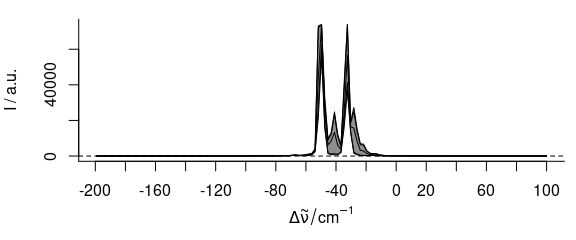
Figure 2.1: The raw laser emission spectra.
As the laser emission was recorded with a Raman spectrometer, the wavelength axis initially is the Raman shift in wavenumbers (cm-1).
As most of the spectra do not show any signal (fig. 2.1), so the spectral range can be cut to -75 – 0 cm-1. Note that negative numbers in the spectral range specification with the tilde do not exclude the spectral range but rather mean negative values of the wavelength axis. The results are shown in figure 2.2.
laser <- laser[, , -75 ~ 0]
plot(laser, "spcprctl5")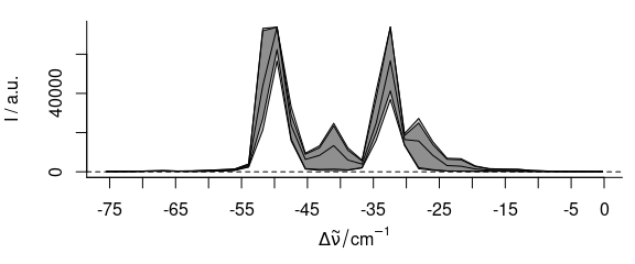
Figure 2.2: The cut spectra laser emission spectra.
The wavelength axis was recorded as Raman shift from 405 nm. However, the spectra were taken before calibrating the wavelength axis. The band at -50 cm-1 is known to be at 405 nm.
Furthermore, as the spectra are not Raman shift but emission, the wavelength axis should be converted to proper wavelengths in nm.
The Raman shift is calculated from the wavelength as follows in equation (2.1) with \(\Delta\tilde\nu\) being the Raman shift, and \(\lambda_0\) the excitation wavelength for a Raman process, here 405 nm.
\[\begin{equation} \Delta\tilde\nu = \frac{1}{\lambda_0} - \frac{1}{\lambda} \tag{2.1} \end{equation}\]
The wavelengths corresponding to the wavenumbers are thus:
\[\begin{equation} \lambda = \frac{1}{ \frac{1}{\lambda_0} - \Delta\tilde\nu} \tag{2.2} \end{equation}\]
Taking into account that 1 cm = 10\(^7\) nm, we arrive at the new wavelength axis:
wl(laser) <- list(
  wl = 1e7 / (1 / 405e-7 - wl(laser)),
  label = expression(lambda / nm)
)
plot(laser, "spcprctl5")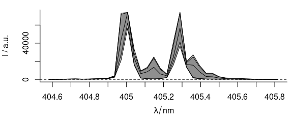
Figure 2.3: The spectra with wavelength axis.
Note that the new wavelength axis label is immediately assigned as well.
laser$filename <- NULL
laser
#> hyperSpec object
#>    84 spectra
#>    2 data columns
#>    36 data points / spectrum
This version of laser datasets is shipped with package hyperSpec.
3 Inspecting the Time Dependency of the Laser Emission
The maxima of the different emission lines encountered during this measurement are at 405.0, 405.1, 405.3, and 405.4 nm (fig. 3.1).
Alternatively they can be extracted from the graph using locator() which reads out the coordinates of the points the user clicks with the mouse (use middle or right click to end the input):
wls <- locator()$x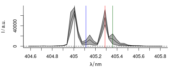
Figure 3.1: The spectral position of the bands in the laser emission time series.
Function plot_c() can also be used to plot time-series.
In that case, the abscissa needs to be specified in parameter use.c.
The collection time is stored in column $t in seconds from start of the measurement, and can be handed over as the column name.
The resulting time series are shown in figure 3.2.
plot_c(laser[, , wls], spc ~ t, groups = .wavelength, type = "b", cex = 0.3, col = cols)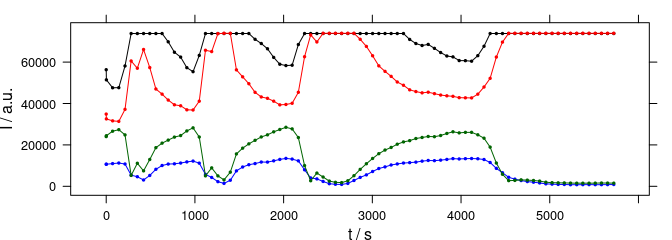
Figure 3.2: The time series data. The colors in this plot correspond to colors in fig. 3.2.
Another option is to condition the plot on \(\lambda\) 3.3.
plot_c(laser[, , wls], spc ~ t | .wavelength, type = "b", cex = 0.3, col = "black")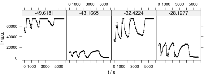
Figure 3.3: The time series plots can also be conditioned on $.wavelength.
4 False-Colour Plot of the Spectral Intensity Over Wavelength and Time
Package hyperSpec supplies functions to draw the spectral matrix using package lattice’s levelplot().
plot(laser, "mat", contour = TRUE, col = "#00000060")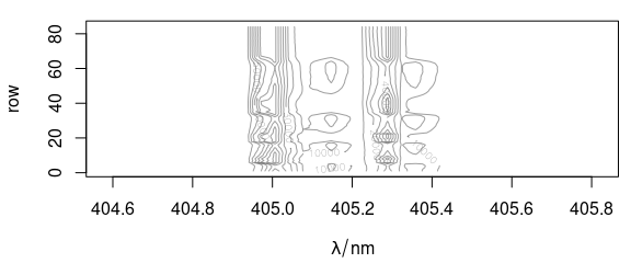
Figure 4.1: The spectra matrix of the laser data set.
The ordinate of the plot may be the number of the spectrum accessed by $.row (here) or any other extra data column, as, e.g., $t in fig. 4.2.
Package hyperSpec’s levelplot() method can be used to display the spectra matrix over a data column (instead of the row number): fig. 4.1, 4.2.
Note that the hyperSpec object is the second argument to the function (according to the notation in levelplot()).
levelplot(spc ~ .wavelength * t, laser, contour = TRUE, col = "#00000080")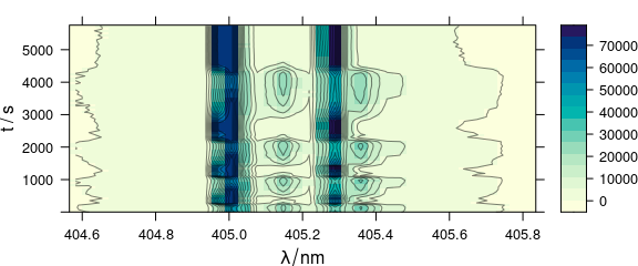
Figure 4.2: The spectra matrix of the laser data set.
The ordinate of the plot may be any extra data column, here $t.
5 A 3D Plot of the Spectral Intensity Over Wavelength and Time
Class hyperSpec objects can be drawn with package rgl[1]:
Package rgl’s function persp3d() plots a surface in 3d defined by points in x, y, and z.
Handing over the appropriate data columns of the hyperSpec object is easy (fig. 5.1).
laser <- laser[, , 404.8 ~ 405.6] / 10000
laser$t <- laser$t / 3600
cols <- rep(matlab.palette(nrow(laser)), nwl(laser))

surface3d(y = wl(laser), x = laser$t, z = laser$spc, col = cols)
surface3d(
  y = wl(laser), x = laser$t, z = laser$spc + .1 * min(laser),
  col = "black", alpha = .2, front = "lines", line_antialias = TRUE
)

aspect3d(c(1, 1, 0.25))

axes3d(c("x+-", "y--", "z--"))
axes3d("y--", nticks = 25, labels = FALSE)
mtext3d("t / h", "x+-", line = 2.5)
mtext3d("lambda / nm", "y--", line = 2.5)
mtext3d("I / a.u.", "z--", line = 2.5)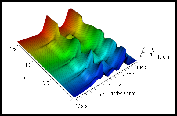
Figure 5.1: The 3d plot of the laser data.
Session Info
sessioninfo::session_info("hyperSpec")
#> ─ Session info ───────────────────────────────────────────────────────────────────────────────────
#>  setting  value
#>  version  R version 4.4.0 (2024-04-24)
#>  os       Ubuntu 22.04.4 LTS
#>  system   x86_64, linux-gnu
#>  ui       X11
#>  language en
#>  collate  C.UTF-8
#>  ctype    C.UTF-8
#>  tz       UTC
#>  date     2024-05-27
#>  pandoc   3.1.11 @ /opt/hostedtoolcache/pandoc/3.1.11/x64/ (via rmarkdown)
#>
#> ─ Packages ───────────────────────────────────────────────────────────────────────────────────────
#>  ! package        * version      date (UTC) lib source
#>    brio             1.1.5        2024-04-24 [2] RSPM
#>    callr            3.7.6        2024-03-25 [2] RSPM
#>    cli              3.6.2        2023-12-11 [2] RSPM
#>    colorspace       2.1-0        2023-01-23 [2] RSPM
#>    crayon           1.5.2        2022-09-29 [2] RSPM
#>    deldir           2.0-4        2024-02-28 [2] RSPM
#>    desc             1.4.3        2023-12-10 [2] RSPM
#>    diffobj          0.3.5        2021-10-05 [2] RSPM
#>    digest           0.6.35       2024-03-11 [2] RSPM
#>    dplyr            1.1.4        2023-11-17 [2] RSPM
#>    evaluate         0.23         2023-11-01 [2] RSPM
#>    fansi            1.0.6        2023-12-08 [2] RSPM
#>    farver           2.1.2        2024-05-13 [2] RSPM
#>    fs               1.6.4        2024-04-25 [2] RSPM
#>    generics         0.1.3        2022-07-05 [2] RSPM
#>    ggplot2        * 3.5.1        2024-04-23 [2] RSPM
#>    glue             1.7.0        2024-01-09 [2] RSPM
#>    gtable           0.3.5        2024-04-22 [2] RSPM
#>    hyperSpec      * 0.200.0.9000 2024-05-27 [1] local
#>    hySpc.testthat   0.2.1        2020-06-24 [2] RSPM
#>    interp           1.1-6        2024-01-26 [2] RSPM
#>    isoband          0.2.7        2022-12-20 [2] RSPM
#>    jpeg             0.1-10       2022-11-29 [2] RSPM
#>    jsonlite         1.8.8        2023-12-04 [2] RSPM
#>    labeling         0.4.3        2023-08-29 [2] RSPM
#>    lattice        * 0.22-6       2024-03-20 [4] CRAN (R 4.4.0)
#>    latticeExtra     0.6-30       2022-07-04 [2] RSPM
#>    lazyeval         0.2.2        2019-03-15 [2] RSPM
#>    lifecycle        1.0.4        2023-11-07 [2] RSPM
#>    magrittr         2.0.3        2022-03-30 [2] RSPM
#>    MASS             7.3-60.2     2024-05-25 [4] local
#>    Matrix           1.7-0        2024-03-22 [4] CRAN (R 4.4.0)
#>    mgcv             1.9-1        2023-12-21 [4] CRAN (R 4.4.0)
#>    munsell          0.5.1        2024-04-01 [2] RSPM
#>    nlme             3.1-164      2023-11-27 [4] CRAN (R 4.4.0)
#>    pillar           1.9.0        2023-03-22 [2] RSPM
#>    pkgbuild         1.4.4        2024-03-17 [2] RSPM
#>    pkgconfig        2.0.3        2019-09-22 [2] RSPM
#>    pkgload          1.3.4        2024-01-16 [2] RSPM
#>    png              0.1-8        2022-11-29 [2] RSPM
#>    praise           1.0.0        2015-08-11 [2] RSPM
#>    processx         3.8.4        2024-03-16 [2] RSPM
#>    ps               1.7.6        2024-01-18 [2] RSPM
#>    R6               2.5.1        2021-08-19 [2] RSPM
#>    RColorBrewer     1.1-3        2022-04-03 [2] RSPM
#>    Rcpp             1.0.12       2024-01-09 [2] RSPM
#>  R RcppEigen        <NA>         <NA>       [?] <NA>
#>    rematch2         2.1.2        2020-05-01 [2] RSPM
#>    rlang            1.1.3        2024-01-10 [2] RSPM
#>    rprojroot        2.0.4        2023-11-05 [2] RSPM
#>    scales           1.3.0        2023-11-28 [2] RSPM
#>    testthat         3.2.1.1      2024-04-14 [2] RSPM
#>    tibble           3.2.1        2023-03-20 [2] RSPM
#>    tidyselect       1.2.1        2024-03-11 [2] RSPM
#>    utf8             1.2.4        2023-10-22 [2] RSPM
#>    vctrs            0.6.5        2023-12-01 [2] RSPM
#>    viridisLite      0.4.2        2023-05-02 [2] RSPM
#>    waldo            0.5.2        2023-11-02 [2] RSPM
#>    withr            3.0.0        2024-01-16 [2] RSPM
#>    xml2             1.3.6        2023-12-04 [2] RSPM
#>
#>  [1] /tmp/RtmpxUEHmP/temp_libpath17ce4b3a89e0
#>  [2] /home/runner/work/_temp/Library
#>  [3] /opt/R/4.4.0/lib/R/site-library
#>  [4] /opt/R/4.4.0/lib/R/library
#>
#>  R ── Package was removed from disk.
#>
#> ──────────────────────────────────────────────────────────────────────────────────────────────────