Calibration- and timeseries plots, depth-profiles and the like
plotc plots intensities of a hyperSpec object over another
dimension such as concentration, time, or a spatial coordinate.
plotc(
  object,
  model = spc ~ c,
  groups = NULL,
  func = NULL,
  func.args = list(),
  ...
)
Arguments
- object
the
hyperSpecobject- model
the lattice model specifying the plot
- groups
grouping variable, e.g.
.wavelengthif intensities of more than one wavelength should be plotted- func
function to compute a summary value from the spectra to be plotted instead of single intensities
- func.args
further arguments to
func- ...
further arguments to
lattice::xyplot().
Details
If func is not NULL, the summary characteristic is calculated
first by applying func with the respective arguments (in
func.args) to each of the spectra. If func returns more than
one value (for each spectrum), the different values end up as different
wavelengths.
If the wavelength is not used in the model specification nor in
groups, nor for specifying subsets, and neither is
func given, then only the first wavelength's intensities are plotted
and a warning is issued.
The special column names .rownames and .wavelength may be used.
The actual plotting is done by lattice::xyplot().
See also
Examples
## example 1: calibration of fluorescence
plotc(flu) ## gives a warning
#> Warning: Intensity at first wavelengh only is used.
 plotc(flu, func = mean)
 plotc(flu, func = range, groups = .wavelength)
 plotc(flu[, , 450], ylab = expression(I["450 nm"] / a.u.))
 calibration <- lm(spc ~ c, data = flu[, , 450]$.)
summary(calibration)
#>
#> Call:
#> lm(formula = spc ~ c, data = flu[, , 450]$.)
#>
#> Residuals:
#> 1 2 3 4 5 6
#> 2.1918 -4.6846 2.1696 1.6005 -1.9306 0.6533
#>
#> Coefficients:
#> Estimate Std. Error t value Pr(>|t|)
#> (Intercept) -8.666 2.876 -3.013 0.0394 *
#> c 2268.482 14.769 153.596 1.08e-08 ***
#> ---
#> Signif. codes: 0 ‘***’ 0.001 ‘**’ 0.01 ‘*’ 0.05 ‘.’ 0.1 ‘ ’ 1
#>
#> Residual standard error: 3.089 on 4 degrees of freedom
#> Multiple R-squared: 0.9998, Adjusted R-squared: 0.9998
#> F-statistic: 2.359e+04 on 1 and 4 DF, p-value: 1.078e-08
#>
plotc(flu[, , 450], type = c("p", "r"))
calibration <- lm(spc ~ c, data = flu[, , 450]$.)
summary(calibration)
#>
#> Call:
#> lm(formula = spc ~ c, data = flu[, , 450]$.)
#>
#> Residuals:
#> 1 2 3 4 5 6
#> 2.1918 -4.6846 2.1696 1.6005 -1.9306 0.6533
#>
#> Coefficients:
#> Estimate Std. Error t value Pr(>|t|)
#> (Intercept) -8.666 2.876 -3.013 0.0394 *
#> c 2268.482 14.769 153.596 1.08e-08 ***
#> ---
#> Signif. codes: 0 ‘***’ 0.001 ‘**’ 0.01 ‘*’ 0.05 ‘.’ 0.1 ‘ ’ 1
#>
#> Residual standard error: 3.089 on 4 degrees of freedom
#> Multiple R-squared: 0.9998, Adjusted R-squared: 0.9998
#> F-statistic: 2.359e+04 on 1 and 4 DF, p-value: 1.078e-08
#>
plotc(flu[, , 450], type = c("p", "r"))
 conc <- list(c = seq(from = 0.04, to = 0.31, by = 0.01))
ci <- predict(calibration, newdata = conc, interval = "confidence", level = 0.999)
panel.ci <- function(x, y, ...,
conc, ci.lwr, ci.upr, ci.col = "#606060") {
panel.xyplot(x, y, ...)
panel.lmline(x, y, ...)
panel.lines(conc, ci.lwr, col = ci.col)
panel.lines(conc, ci.upr, col = ci.col)
}
plotc(flu[, , 450],
panel = panel.ci,
conc = conc$c, ci.lwr = ci[, 2], ci.upr = ci[, 3]
)
conc <- list(c = seq(from = 0.04, to = 0.31, by = 0.01))
ci <- predict(calibration, newdata = conc, interval = "confidence", level = 0.999)
panel.ci <- function(x, y, ...,
conc, ci.lwr, ci.upr, ci.col = "#606060") {
panel.xyplot(x, y, ...)
panel.lmline(x, y, ...)
panel.lines(conc, ci.lwr, col = ci.col)
panel.lines(conc, ci.upr, col = ci.col)
}
plotc(flu[, , 450],
panel = panel.ci,
conc = conc$c, ci.lwr = ci[, 2], ci.upr = ci[, 3]
)
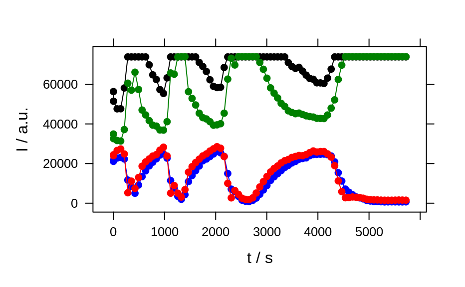
 ## example 2: time-trace of laser emission modes
cols <- c("black", "blue", "#008000", "red")
wl <- i2wl(laser, c(13, 17, 21, 23))
plot_spc(laser, axis.args = list(x = list(at = seq(404.5, 405.8, .1))))
for (i in seq_along(wl)) {
abline(v = wl[i], col = cols[i], lwd = 2)
}
## example 2: time-trace of laser emission modes
cols <- c("black", "blue", "#008000", "red")
wl <- i2wl(laser, c(13, 17, 21, 23))
plot_spc(laser, axis.args = list(x = list(at = seq(404.5, 405.8, .1))))
for (i in seq_along(wl)) {
abline(v = wl[i], col = cols[i], lwd = 2)
}
 plotc(laser[, , wl], spc ~ t,
groups = .wavelength, type = "b",
col = cols
)
plotc(laser[, , wl], spc ~ t,
groups = .wavelength, type = "b",
col = cols
)