Introduction to unmixR

Hyperspectral Unmixing

Bryan A. Hanson

July 29, 2016

This vignette provides a general background on hyperspectral unmixing. The unmixR package provides several other vignettes that detail each of the main algorithms available in the package. You can access them as follows:

library("unmixR")
browseVignettes("unmixR")

What are Hyperspectral Data?

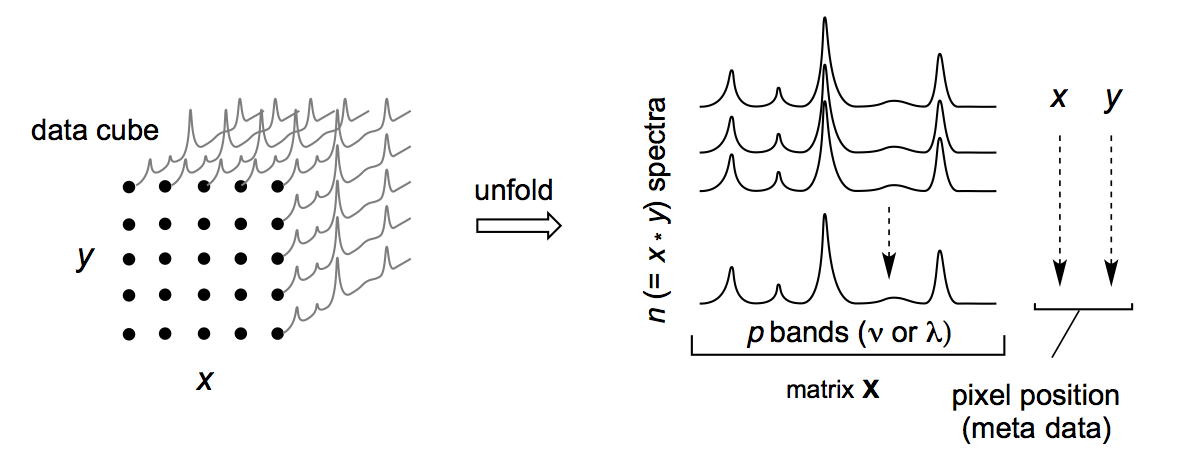
Hyperspectral data are spectroscopic data collected in a spatial or temporal context. Each sample is a spectrum collected at a particular location or time. Each spectrum is thus accompanied by meta-data giving this information, which is needed to reconstruct images and for other types of analysis. The following figure illustrates the nature of a typical data set. Note that while data is often collected on an \(x,y\) grid, it need not be.

DataCube

Examples of Hyperspectral Data Sets

Hyperspectral data sets are encountered in many disciplines. Here are some examples of hyperspectral data sets.

• Biomedical imaging: a series of Raman spectra are collected as a microscopic piece of tissue is scanned in an \(x,y\) plane. Such studies are of interest for real time imaging of surgical tissue samples. Other types of spectroscopy can be employed, for instance mass spectrometry.^1  2

• Airborne imaging: A satellite, plane or drone flies a pattern over land and collects spectra in the visible, UV or NIR range. Such studies have been used to map mineral formations and to study the quality of forest canopies.^3  4

• Art history: A painting is scanned to examine the underlying pigments and perhaps reveal the presence of additional hidden images.⁵

What is Meant by Unmixing?

Unmixing is the process of taking a data set such as those described above and extracting the pure spectra that make up the data. For instance, a mineral-rich landscape may have regions that consist of pure minerals and regions where minerals are mixed due to erosion and movement of materials. Pure minerals have characteristic IR spectra. Spectra collected as part of an airborne imaging study of the region would be expected to consist of many spectral mixtures as well as some pure or nearly pure spectra.

Terminology: Since so many applications involve collecting data over a \(x,y\) grid, this is often referred to as an image or “scene”. This scene is often said to be composed to “pixels” which would correspond to the sample spectra. The pure component spectra are typically referred to as “endmembers.” Sometimes they are simply called components.

What Information Can Be Obtained?

• Endmembers: The pure spectra of the components of the scene. These can be compared to databases or analyzed using the appropriate domain knowledge to determine their identity.

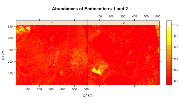
• Abundances: Once the endmembers have been obtained, they can be used to calculate the abundances of each endmember at each point in the scene. From this, one can make an abundance map. In the mineral-rich landscape example, this could be a map of a particular mineral of interest.

An Example

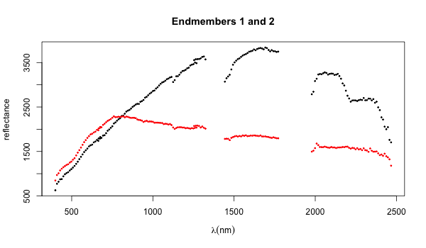
Much of the hyperspectral unmixing literature comes from the field of remote sensing where airborne platforms are employed to collect the data. The mineral-rich landscape example above is not an abstraction. A frequently used example is the AVIRIS study of the cuprite region in the state of Nevada, USA. This region is devoid of most vegetation and rich in geological formations.⁶

The following results are based on unmixing a small portion of the cuprite data set. The first figure shows two of the endmembers (careful work and comparison to ground-based geological studies suggest that there are at least 19 distinct mineral entities present). Using the appropriate domain knowledge these endmembers can be identified.

endmembers

The next figure is an abundance map of these endmembers. Clearly if you were a prospector these maps would be a great guide to finding treasure!

abundance map

The Unmixing Process

Algebraic Description of the Data

In the following, lower-case bold letters represent vectors (matrices with a single row or column), e.g. \(\mathbf{x}\). The corresponding upper-case letter, \(\mathbf{X}\), represents the same conceptual quantity, but scaled up so that each dimension is greater than 1. Since hyperspectral data sets are typically stored with samples in rows and wavelengths in columns, \(\mathbf{x}\) would be a particular row of \(\mathbf{X}\).

For hyperspectral data measured at \(p\) wavelengths, and assuming \(m\) endmembers are present, the data in a hyperspectral study can be represented in several ways. A single sample is a spectrum at location (pixel) or time point. It can be represented as

\[ \mathbf{x}^{(1 \ \times \ p)} = \mathbf{a}^{(1 \ \times \ m)} \times \mathbf{E}^{(m \ \times \ p)} + \epsilon \]

Where \(\mathbf{x}\) is the spectrum, \(\mathbf{a}\) gives the fraction of each endmember present at that particular pixel, and \(\mathbf{E}\) is a matrix of the endmembers, the pure component spectra. \(\epsilon\) represents noise. Think of \(\mathbf{E}\) as a library of reference spectra. It’s just that before unmixing you don’t have that library! In words, this says that a given spectrum is the sum of the product of each abundance times the corresponding reference spectrum, plus noise.

If we scale this up to a real data set containing \(n\) samples, the equation above becomes

\[ \mathbf{X}^{(n \ \times \ p)} = \mathbf{A}^{(n \ \times \ m)} \times \mathbf{E}^{(m \ \times \ p)} + \epsilon \]

where \(\mathbf{X}\) is a matrix of the raw data and \(\mathbf{A}\) is a matrix giving the abundances of each endmember in each sample (\(\mathbf{E}\) and \(\epsilon\) as before). If we drop some of the extra notation, the above can be written

\[ \mathbf{X} = \mathbf{A}\mathbf{E} + \epsilon \]

for simplicity.

If instead we scale down to a single wavelength in a single spectrum, the equation becomes

\[ x_k = \mathbf{a} \times \mathbf{e}_k \]

where \(k\) is one of the \(p\) wavelengths (\(\mathbf{e}_k\) is one wavelength selected from the reference library \(\mathbf{E}\)).

By the way, this way of looking at the data is called the “linear mixing model” or the “convex geometry model.” We’ll have more to say about this latter term in a bit.

The system is subject to several constraints. The abundances must be positive, and they must sum to one.

\[ 0 \leqq a_i \leqq 1 \]

\[ \sum_{i=1}^{m} a_i = 1 \]

where \(i\) is one of the \(m\) endmembers of the system.

Data Reduction

All hyperspectral unmixing algorithms begin with some sort of data reduction step. There are several possibilities, but the most familiar will be PCA or principal components analysis. PCA is a widely used method which converts raw data into uncorrelated abstract components which can stand in for the data. The advantage to this is that you don’t need all the components to represent the data, because some or even many of them are merely noise. In the spectral context, this is equivalent to saying that some wavelengths are not informative, so we can discard them with little change to our analysis. PCA is a dimensional reduction method because instead of having \(p\) wavelengths, we now have many fewer abstract components to deal with. Hence PCA not only removes noise but makes the problem computationally much faster.

After PCA (or a similar technique), the equation describing the system would be:

\[ \mathbf{X} = \mathbf{A}\mathbf{E} \]

where \(\epsilon\) has effectively been eliminated. However, and this is important, \(\mathbf{X}\) is no longer the original data, but rather the abstract components. Its dimensions are still \(n \ \times \ p\), but \(p\) is no longer \(p\), it is much smaller than the original number of wavelengths. Perhaps it should be called something different, like \(p'\), but the habit in the literature is to ignore that \(\mathbf{X}\) and \(p\) are no longer what they were originally. The subsequent steps apply either way, but after dimension reduction they are computationally tractable.

The Role of the Simplex

A key concept common to unmixing algorithms is that of a simplex. A simplex is a container that holds the data points. For two-dimensional data (measurements at two wavelengths), such as that illustrated below, several kinds of containers can be imagined. The “convex hull” is a container that is shrink-wrapped around the cloud of data points. A simplex for two-dimensional data is a scalene triangle of the smallest possible size.

2-Simplex

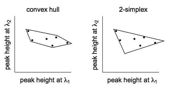
The reason a simplex is of interest is that for unmixing purposes, the vertices of the simplex are the locations of the endmembers. Sticking with the two-dimensional example, the three vertices correspond theoretically to pure components. Every other point inside the simplex can be thought of as a weighted average of each of the endmembers.

If one has spectra composed of \(p\) wavelengths, the data exists as a point cloud in \(p\)-dimensions. If \(p = 2\) as in the figure above, the cloud of data can be captured in a 2-simplex or triangle. For \(p = 3\), a tetrahedron would be needed to contain the data. For \(p > 3\) there is no simple visual analog to the container, but we know that it would have \(p + 1\) edges. Typical data sets might have hundreds or even thousands of wavelengths. Simplices of this size are hard to imagine and would be computationally intractable regardless. Recall from the section above however, that prior to the unmixing process, we reduce the data (remember that \(p\) is not really \(p\) any longer). Thus, a data set of perhaps hundreds of wavelengths can be reduced to a much smaller dimensionality. In practice, \(p\) is chosen (or perhaps we should say “guessed at”) by the researcher using the relevant domain knowledge. The unmixing process then seeks to find these \(p\) endmembers from which all the data can be reconstructed.

Algorithm Options

With this background in mind, you should be ready to read the vignettes on individual algorithms. A number of unmixing algorithms have been described in the literature. The chief difference between them is how they go about finding the relevant simplex. In unmixR, there are variations of the NFINDR, VCA and ICE algorithms. See ?nfindr, ?vca, ?ice or browseVignettes("unmixR") for additional information.

Project History

The development of unmixR was initiated by Claudia Beleites. Most of the code was written by Conor McManus (2013) and Anton Belov (2016). Conor and Anton were participants in the Google Summer of Code program. Additional code was written by Claudia and Bryan A. Hanson. Claudia, Bryan and Simon Fuller were the mentors in the GSOC program.

Notes

1 Bergner et. al. “Hyperspectral unmixing of Raman micro-images for assessment of morphological and chemical parameters in non-dried brain tumor specimens” Anal. Bioanalytical Chemistry vol. 405 no. 27 pp. 8719-8728 (2013).↵

2 Hedegaard et. al. “Spectral unmixing and clustering algorithms for assessment of single cells by Raman microscopic imaging” Theoretical Chemistry Accounts vol. 130 no. 4-6 pp. 1249-1260 (2011).↵

3 Green et. al. “Imaging spectroscopy and the Airborne Visible Infrared Imaging Spectrometer (AVIRIS)” Remote Sensing Environment vol. 65 no. 3 pp. 227-248 (1998).↵

4 Jetz et. al. “Monitoring plant functional diversity from space” Nature Plants vol. 2 no. 3 pp. ? (2016).↵

5 Dooley et. al “Mapping of egg yolk and animal skin glue paint binders in Early Renaissance paintings using near infrared reflectance imaging spectroscopy” Analyst vol. 138 no. 17 pp. 4838-4848 (2013).↵

6 Green1998 op. cit. ↵

GSOC Logo