Calibration of Quinine Fluorescence Emission
Example Workflow for Fluorescence Emission Dataset flu
Claudia Beleites1,2,3,4,5, Vilmantas Gegzna
- DIA Raman Spectroscopy Group, University of Trieste/Italy (2005–2008)
- Spectroscopy \(\cdot\) Imaging, IPHT, Jena/Germany (2008–2017)
- ÖPV, JKI, Berlin/Germany (2017–2019)
- Arbeitskreis Lebensmittelmikrobiologie und Biotechnologie, Hamburg University, Hamburg/Germany (2019 – 2020)
- Chemometric Consulting and Chemometrix GmbH, Wölfersheim/Germany (since 2016)
chemometrie@beleites.de
2024-05-27
Source:vignettes/flu.Rmd
flu.Rmd
list.files(system.file("doc/rawdata", package = "hyperSpec"), pattern = "flu[1-6][.]txt")This tutorial provides an example of how to:
- Write an import function for proprietary ASCII files from a spectrometer manufacturer.
- Add additional data columns to the spectra.
- Set up a linear calibration (inverse least squares).
The flu dataset in the hyperSpec package consists of six fluorescence emission spectra of quinine solutions.
These spectra were acquired during a student practicum and were kindly provided by M. Kammer.
The concentrations of the solutions range from 0.05 to 0.30 mg/l, and the spectra were acquired using a Perkin Elmer LS50-B fluorescence spectrometer at 350 nm excitation.
1 Writing an Import Function
The raw spectra are stored in Perkin Elmer’s ASCII file format, with one spectrum per file. These files are completely ASCII text, and the actual spectra start at line 55.
The function to import these files, read.txt.PerkinElmer(), is discussed in the “fileIO” vignette, please refer to that document for details.
It needs to be source()d before use:
source("read.txt.PerkinElmer.R")

folder <- system.file("extdata/flu", package = "hyperSpec")
files <- Sys.glob(paste0(folder, "/flu?.txt"))
flu <- read.txt.PerkinElmer(files, skip = 54)
Now, the spectra are contained within a hyperSpec object and can be examined, e.g., by:
flu
#> hyperSpec object
#>    6 spectra
#>    2 data columns
#>    181 data points / spectrum
plot(flu)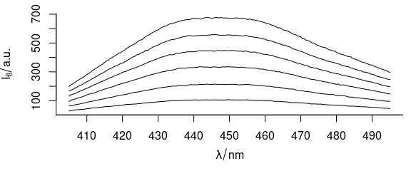
Figure 1.1: Six spectra of flu dataset.
2 Adding Further Data Columns
The calibration model requires the quinine concentrations for the spectra. This information can be stored alongside the spectra and also gets an appropriate label:
flu$c <- seq(from = 0.05, to = 0.30, by = 0.05)
labels(flu, "c") <- "c, mg/l"

flu
#> hyperSpec object
#>    6 spectra
#>    3 data columns
#>    181 data points / spectrum
save(flu, file = "flu.rda")Now, the hyperSpec object flu contains two data columns, holding the actual spectra and the respective concentrations. The dollar operator returns such a data column:
flu$c
#> [1] 0.05 0.10 0.15 0.20 0.25 0.30
3 Dropping data columns
Function read.txt.PerkinElmer() added a column with the file names that we don’t need.
flu$..
#>                                                                  filename    c
#> 1 /tmp/RtmpxUEHmP/temp_libpath17ce4b3a89e0/hyperSpec/extdata/flu/flu1.txt 0.05
#> 2 /tmp/RtmpxUEHmP/temp_libpath17ce4b3a89e0/hyperSpec/extdata/flu/flu2.txt 0.10
#> 3 /tmp/RtmpxUEHmP/temp_libpath17ce4b3a89e0/hyperSpec/extdata/flu/flu3.txt 0.15
#> 4 /tmp/RtmpxUEHmP/temp_libpath17ce4b3a89e0/hyperSpec/extdata/flu/flu4.txt 0.20
#> 5 /tmp/RtmpxUEHmP/temp_libpath17ce4b3a89e0/hyperSpec/extdata/flu/flu5.txt 0.25
#> 6 /tmp/RtmpxUEHmP/temp_libpath17ce4b3a89e0/hyperSpec/extdata/flu/flu6.txt 0.30
It is therefore deleted:
flu$filename <- NULL4 Linear Calibration
As R is developed for statistical analysis, tools for a least squares calibration model are readily available.
The original spectra range from 405 to 495 nm. However, the intensities at 450 nm are perfect for a univariate calibration. Plotting them against the concentration can be done as follows:
plot_c(flu[, , 450])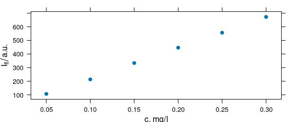
Figure 4.1: Spectra intensities at 450 nm.
The square bracket operator extracts parts of a hyperSpec object.
The first coordinate defines which spectra are to be used, the second which data columns, and the third gives the spectral range.
We discard all the wavelengths but 450 nm:
flu <- flu[, , 450]
labels(flu, "spc") <- expression(I["450 nm"] / a.u.)
The plot could be enhanced by annotating the ordinate with the emission wavelength. Also the axes should start at the origin, so that it is easier to see whether the calibration function will go through the origin:
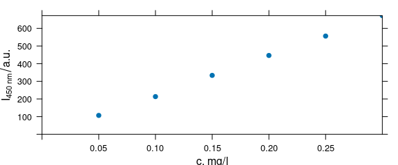
Figure 4.2: Spectra intensities at 450 nm with updated labels.
The actual calibration is a linear model, which can be fitted by the R function lm().
The function lm() needs a formula that specifies which data columns are dependent and independent variables.
The normal calibration plot gives the emission intensity as a function of the concentration, and the calibration function thus models \(I = f (c)\), i. e. \(I = m c + b\) for a linear calibration. This is then solved for \(c\) when the calibration is used.
However, R’s linear model is a quite strict in predicting: a model set up as \(I = f (c)\) will predict the intensity as a function of the concentration but not the other way round.
Thus we set up an inverse calibration model[^As we can safely assume that the error on the concentrations is far larger than the error on the instrument signal, it is actually the correct type of model from the least squares fit point of view.]: \(c = f (I)\).
The corresponding formula is c ~ I, or in our case c ~ spc, as the intensities are stored in the data column $spc:
In addition, lm() (like most R model building functions) expects the data to be a data.frame.
There are three abbreviations that help to get the parts of the hyperSpec object that are frequently needed:
-
flu[[]]returns the spectra matrix. It takes the same indices as[]. -
flu\$.returns the data as adata.frame. -
flu\$..returns adata.framethat has all data columns but the spectra.
flu[[]]
#>         450
#> [1,] 106.95
#> [2,] 213.50
#> [3,] 333.78
#> [4,] 446.63
#> [5,] 556.52
#> [6,] 672.53
flu$.
#>      450    c
#> 1 106.95 0.05
#> 2 213.50 0.10
#> 3 333.78 0.15
#> 4 446.63 0.20
#> 5 556.52 0.25
#> 6 672.53 0.30
flu$..
#>      c
#> 1 0.05
#> 2 0.10
#> 3 0.15
#> 4 0.20
#> 5 0.25
#> 6 0.30
Putting this together, the calibration model is calculated:
calibration <- lm(c ~ spc, data = flu$.)The summary() gives a good overview of our model:
summary(calibration)
#>
#> Call:
#> lm(formula = c ~ spc, data = flu$.)
#>
#> Residuals:
#>         1         2         3         4         5         6
#> -0.000987  0.002052 -0.000960 -0.000701  0.000864 -0.000267
#>
#> Coefficients:
#>             Estimate Std. Error t value Pr(>|t|)
#> (Intercept) 3.85e-03   1.25e-03    3.09    0.037 *
#> spc         4.41e-04   2.87e-06  153.60  1.1e-08 ***
#> ---
#> Signif. codes:  0 '***' 0.001 '**' 0.01 '*' 0.05 '.' 0.1 ' ' 1
#>
#> Residual standard error: 0.00136 on 4 degrees of freedom
#> Multiple R-squared:     1,   Adjusted R-squared:     1
#> F-statistic: 2.36e+04 on 1 and 4 DF,  p-value: 1.08e-08
In order to get predictions for new measurements, a new data.frame with the same independent variables (in columns with the same names) as in the calibration data are needed.
Then the function predict() can be used.
It can also calculate the prediction interval.
If we observe e.g. an intensity of 125 or 400 units, the corresponding concentrations and their 99% prediction intervals are:
I <- c(125, 400)
conc <- predict(calibration,
  newdata = list(spc = as.matrix(I)), interval = "prediction",
  level = .99
)
conc
#>        fit     lwr      upr
#> 1 0.058943 0.05133 0.066556
#> 2 0.180149 0.17338 0.186922
Finally, we can draw the calibration function and its 99% confidence interval (also via predict()) together with the prediction example.
In order to draw the confidence interval into the calibration graph, we can either use a customized panel function:
int <- list(spc = as.matrix(seq(min(flu), max(flu), length.out = 25)))
ci <- predict(calibration, newdata = int, interval = "confidence", level = 0.99)

panel.ci <- function(x, y, ..., intensity, ci.lwr, ci.upr, ci.col = "#606060") {
  panel.xyplot(x, y, ...)
  panel.lmline(x, y, ...)
  panel.lines(ci.lwr, intensity, col = ci.col)
  panel.lines(ci.upr, intensity, col = ci.col)
}

plot_c(flu,
  panel = panel.ci,
  intensity = int$spc, ci.lwr = ci[, 2], ci.upr = ci[, 3]
)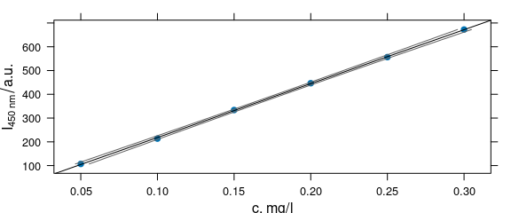
Figure 4.3: Calibration function and its 99% confidence interval.
Or, we can add the respective data to the hyperSpec object. The meaning of the data can be saved in a new extra data column that acts as grouping variable for the plot.
First, the spectral range of flu is cut to contain the fluorescence emission at 450 nm only, and the new column is introduced for the original data:
flu$type <- "data points"Next, the calculated confidence intervals are appended:
tmp <- new("hyperSpec",
  spc = as.matrix(seq(min(flu), max(flu), length.out = 25)),
  wavelength = 450
)
ci <- predict(calibration, newdata = tmp$., interval = "confidence", level = 0.99)
tmp <- tmp[rep(seq(tmp, index = TRUE), 3)]
tmp$c <- as.numeric(ci)
tmp$type <- rep(colnames(ci), each = 25)

flu <- collapse(flu, tmp)
Finally, the resulting object is plotted. Our prediction example is handled by another customized panel function:
panel.predict <-
  function(x, y, ..., intensity, ci, pred.col = "red", pred.pch = 19, pred.cex = 1) {
    panel.xyplot(x, y, ...)
    mapply(
      function(i, lwr, upr, ...) {
        panel.lines(c(lwr, upr), rep(i, 2), ...)
      },
      intensity, ci[, 2], ci[, 3],
      MoreArgs = list(col = pred.col)
    )
    panel.xyplot(ci[, 1], intensity, col = pred.col, pch = pred.pch, cex = pred.cex, type = "p")
  }

plot_c(flu,
  groups = type, type = c("l", "p"),
  col = c("black", "black", "#606060", "#606060"),
  pch = c(19, NA, NA, NA),
  cex = 0.5,
  lty = c(0, 1, 1, 1),
  panel = panel.predict,
  intensity = I,
  ci = conc,
  pred.cex = 0.5
)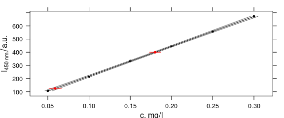
Figure 4.4: calibration function and its 99% confidence interval and predicted points.
Session Info
sessioninfo::session_info("hyperSpec")
#> ─ Session info ───────────────────────────────────────────────────────────────────────────────────
#>  setting  value
#>  version  R version 4.4.0 (2024-04-24)
#>  os       Ubuntu 22.04.4 LTS
#>  system   x86_64, linux-gnu
#>  ui       X11
#>  language en
#>  collate  C.UTF-8
#>  ctype    C.UTF-8
#>  tz       UTC
#>  date     2024-05-27
#>  pandoc   3.1.11 @ /opt/hostedtoolcache/pandoc/3.1.11/x64/ (via rmarkdown)
#>
#> ─ Packages ───────────────────────────────────────────────────────────────────────────────────────
#>  ! package        * version      date (UTC) lib source
#>    brio             1.1.5        2024-04-24 [2] RSPM
#>    callr            3.7.6        2024-03-25 [2] RSPM
#>    cli              3.6.2        2023-12-11 [2] RSPM
#>    colorspace       2.1-0        2023-01-23 [2] RSPM
#>    crayon           1.5.2        2022-09-29 [2] RSPM
#>    deldir           2.0-4        2024-02-28 [2] RSPM
#>    desc             1.4.3        2023-12-10 [2] RSPM
#>    diffobj          0.3.5        2021-10-05 [2] RSPM
#>    digest           0.6.35       2024-03-11 [2] RSPM
#>    dplyr            1.1.4        2023-11-17 [2] RSPM
#>    evaluate         0.23         2023-11-01 [2] RSPM
#>    fansi            1.0.6        2023-12-08 [2] RSPM
#>    farver           2.1.2        2024-05-13 [2] RSPM
#>    fs               1.6.4        2024-04-25 [2] RSPM
#>    generics         0.1.3        2022-07-05 [2] RSPM
#>    ggplot2        * 3.5.1        2024-04-23 [2] RSPM
#>    glue             1.7.0        2024-01-09 [2] RSPM
#>    gtable           0.3.5        2024-04-22 [2] RSPM
#>    hyperSpec      * 0.200.0.9000 2024-05-27 [1] local
#>    hySpc.testthat   0.2.1        2020-06-24 [2] RSPM
#>    interp           1.1-6        2024-01-26 [2] RSPM
#>    isoband          0.2.7        2022-12-20 [2] RSPM
#>    jpeg             0.1-10       2022-11-29 [2] RSPM
#>    jsonlite         1.8.8        2023-12-04 [2] RSPM
#>    labeling         0.4.3        2023-08-29 [2] RSPM
#>    lattice        * 0.22-6       2024-03-20 [4] CRAN (R 4.4.0)
#>    latticeExtra     0.6-30       2022-07-04 [2] RSPM
#>    lazyeval         0.2.2        2019-03-15 [2] RSPM
#>    lifecycle        1.0.4        2023-11-07 [2] RSPM
#>    magrittr         2.0.3        2022-03-30 [2] RSPM
#>    MASS             7.3-60.2     2024-05-25 [4] local
#>    Matrix           1.7-0        2024-03-22 [4] CRAN (R 4.4.0)
#>    mgcv             1.9-1        2023-12-21 [4] CRAN (R 4.4.0)
#>    munsell          0.5.1        2024-04-01 [2] RSPM
#>    nlme             3.1-164      2023-11-27 [4] CRAN (R 4.4.0)
#>    pillar           1.9.0        2023-03-22 [2] RSPM
#>    pkgbuild         1.4.4        2024-03-17 [2] RSPM
#>    pkgconfig        2.0.3        2019-09-22 [2] RSPM
#>    pkgload          1.3.4        2024-01-16 [2] RSPM
#>    png              0.1-8        2022-11-29 [2] RSPM
#>    praise           1.0.0        2015-08-11 [2] RSPM
#>    processx         3.8.4        2024-03-16 [2] RSPM
#>    ps               1.7.6        2024-01-18 [2] RSPM
#>    R6               2.5.1        2021-08-19 [2] RSPM
#>    RColorBrewer     1.1-3        2022-04-03 [2] RSPM
#>    Rcpp             1.0.12       2024-01-09 [2] RSPM
#>  R RcppEigen        <NA>         <NA>       [?] <NA>
#>    rematch2         2.1.2        2020-05-01 [2] RSPM
#>    rlang            1.1.3        2024-01-10 [2] RSPM
#>    rprojroot        2.0.4        2023-11-05 [2] RSPM
#>    scales           1.3.0        2023-11-28 [2] RSPM
#>    testthat         3.2.1.1      2024-04-14 [2] RSPM
#>    tibble           3.2.1        2023-03-20 [2] RSPM
#>    tidyselect       1.2.1        2024-03-11 [2] RSPM
#>    utf8             1.2.4        2023-10-22 [2] RSPM
#>    vctrs            0.6.5        2023-12-01 [2] RSPM
#>    viridisLite      0.4.2        2023-05-02 [2] RSPM
#>    waldo            0.5.2        2023-11-02 [2] RSPM
#>    withr            3.0.0        2024-01-16 [2] RSPM
#>    xml2             1.3.6        2023-12-04 [2] RSPM
#>
#>  [1] /tmp/RtmpxUEHmP/temp_libpath17ce4b3a89e0
#>  [2] /home/runner/work/_temp/Library
#>  [3] /opt/R/4.4.0/lib/R/site-library
#>  [4] /opt/R/4.4.0/lib/R/library
#>
#>  R ── Package was removed from disk.
#>
#> ──────────────────────────────────────────────────────────────────────────────────────────────────