Plotting “hyperSpec” with “ggplot2”
Claudia Beleites1,2,3,4,5, Vilmantas Gegzna
- DIA Raman Spectroscopy Group, University of Trieste/Italy (2005–2008)
- Spectroscopy \(\cdot\) Imaging, IPHT, Jena/Germany (2008–2017)
- ÖPV, JKI, Berlin/Germany (2017–2019)
- Arbeitskreis Lebensmittelmikrobiologie und Biotechnologie, Hamburg University, Hamburg/Germany (2019 – 2020)
- Chemometric Consulting and Chemometrix GmbH, Wölfersheim/Germany (since 2016)
chemometrie@beleites.de
2023-04-23
Source:vignettes/hySpc-ggplot2.Rmd
hySpc-ggplot2.RmdSuggested Packages and Setup
Reproducing the examples in this vignette.
All spectra used in this manual are installed automatically with package hyperSpec.
Terminology Throughout the documentation of the package, the following terms are used:
- wavelength indicates any type of spectral abscissa.
- intensity indicates any type of spectral ordinate.
- extra data indicates non-spectroscopic data.
Using ggplot2 with hyperSpec objects
Class hyperSpec[R-hyperSpec?] objects do not yet directly support plotting with package ggplot2[1,R-ggplot2?].
Nevertheless, package ggplot2 graphics can easily be obtained by using qplot*() equivalents to hyperSpec::plot_spc(), hyperSpec::plotc(), and hyperSpec::plotmap().
Function qplotspc()
Plot spectra with qplotspc() (Fig. 1).
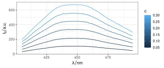
Figure 1: Spectra produced by qplotspc(): flu data.
qplotspc(paracetamol, c(2800 ~ max, min ~ 1800)) +
  scale_x_reverse(breaks = seq(0, 3200, 400))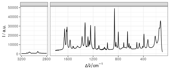
Figure 2: Spectra with reversed order of x axis values: paracetamol data.
Let’s look at the other dataset called faux_cell.
set.seed(1)
faux_cell <- generate_faux_cell()
faux_cell
#> hyperSpec object
#>    875 spectra
#>    4 data columns
#>    300 data points / spectrum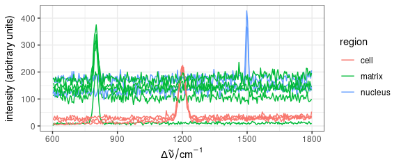
Figure 3: Ten randomly selected spectra from faux_cell dataset.
Average spectra of each region.
qplotspc(
  aggregate(faux_cell, faux_cell$region, mean),
  mapping = aes(x = .wavelength, y = spc, colour = region)
) +
  facet_grid(region ~ .)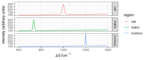
Figure 4: Mean spectra of each region in faux_cell dataset.
Mean \(\pm\) standard deviation:
qplotspc(
  aggregate(faux_cell, faux_cell$region, mean_pm_sd),
  mapping = aes(x = .wavelength, y = spc, colour = region, group = .rownames)
) +
  facet_grid(region ~ .)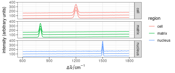
Figure 5: Mean \(\pm\) standard deviation spectra of each region in faux_cell dataset.
Function qplotc()
This function plots spectroscopic concenration, depth, time-series, etc. profiles.
By default, plots spectrum only at the first wavelength.
qplotc(flu)
#> Warning in qplotc(flu): Intensity at first wavelengh only is used.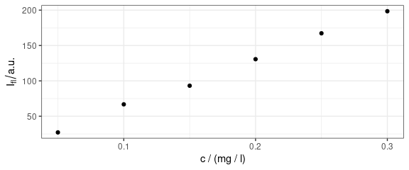
Figure 6: Concentration profile: intensities at the first available wavelength value.
It is better to indicate the wavelength of interest explicitly.
qplotc(flu[, , 410])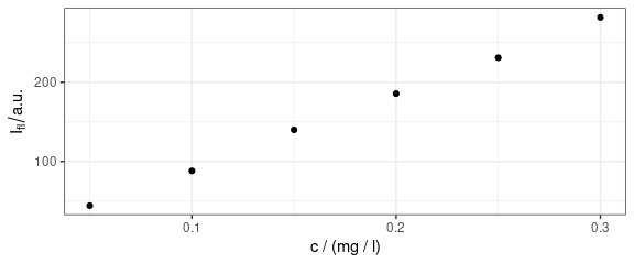
Figure 7: Concentration profile: intensities at 410 nm.
qplotc(flu[, , 410]) +
  geom_smooth(method = "lm", formula = y ~ x)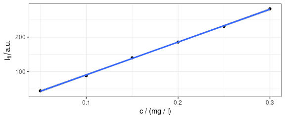
Figure 8: Concentration profile with fitted line.
Function ggplotmap()
Fig. 9 shows a map created with package ggplot2.
set.seed(7)
faux_cell <- generate_faux_cell()
qplotmap(faux_cell[, , 1200])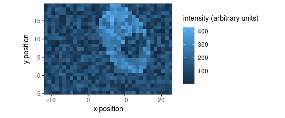
Figure 9: False-colour map produced by qplotmap().
qplotmap(faux_cell[, , 1200]) +
  scale_fill_gradientn("Intensity", colours = palette_matlab())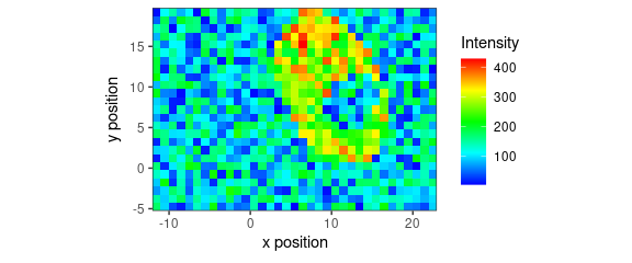
Figure 10: False-colour map produced by qplotmap(): different color palette.
If you have package viridis installed, you may try:
qplotmap(faux_cell[ , , 1200]) +
    viridis::scale_fill_viridis("Intensity")
The two special columns .wavelength and .rownames contain the wavelength axis and allow to distinguish the spectra.
Function qplotmixmap()
This function plots false-colour map with colour mixing for multivariate overlay.
set.seed(1)
faux_cell <- generate_faux_cell()
Without pre-processing:
qplotmixmap(faux_cell[, , c(800, 1200, 1500)],
  purecol = c(matrix = "red", cell = "green", nucleus = "blue")
)
#> Warning: Removed 300 rows containing missing values (`geom_point()`).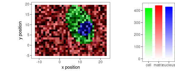
Figure 11: False-color map produced by qplotmixmap(): raw faux_cell spectra at 800, 1200, and 1500 \(cm^{-1}.\)
With baseline removed:
faux_cell_2 <- faux_cell - spc_fit_poly_below(faux_cell)

qplotmixmap(faux_cell_2[, , c(800, 1200, 1500)],
  purecol = c(matrix = "red", cell = "green", nucleus = "blue")
)
#> Warning: Removed 300 rows containing missing values (`geom_point()`).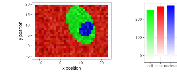
Figure 12: False-color map of faux_cell spectra with base line removed.
With some further pre-processing:
faux_cell_3 <- faux_cell_2
faux_cell_3 <- sweep(faux_cell_3, 1, apply(faux_cell_3, 1, mean), "/")
faux_cell_3 <- sweep(faux_cell_3, 2, apply(faux_cell_3, 2, quantile, 0.05), "-")

qplotmixmap(faux_cell_3[, , c(800, 1200, 1500)],
  purecol = c(matrix = "red", cell = "green", nucleus = "blue")
)
#> Warning: Removed 300 rows containing missing values (`geom_point()`).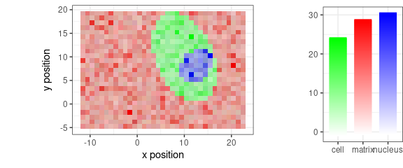
Figure 13: False-color map of pre-processed faux_cell spectra.
More General Plotting with ggplot2
For more general plotting, as.long.df() transforms a hyperSpec object into a long-form data.frame that is suitable for qplot(), while as.t.df() produces a data.frame where each spectrum is one column, and an additional first column gives the wavelength.
Long data.frames can be very memory consuming as they are of size \(nrow · nwl × (ncol + 2)\) with respect to the dimensions of the hyperSpec object.
Thus, e.g., the faux_cell data set (2 MB) as hyperSpec object) needs 26 MB as long-format data.frame.
It is therefore highly recommended to calculate the particular data to be plotted beforehand.
qplotspc(mean(faux_cell)) +
  geom_ribbon(
    aes(
      ymin = mean + sd,
      ymax = mean - sd,
      y = 0,
      group = NA
    ),
    alpha = 0.25,
    data = as.t.df(mean_sd(faux_cell))
  )
Note that qpotspc() specifies aesthetics y = spc and groups = .rownames, which do not have corresponding columns in the data.frame returned by as.t.df().
These aesthetics must therefore be set manually in the aesthetics definition in geom_ribbon() (or any other geom_*() that uses as.t.df()).
Otherwise, errors occur that object spc (and/or .rownames) cannot be found.
Cut axes can be implemented by faceting (Fig. 14).
qplotspc(paracetamol / 1e4, wl.range = c(min ~ 1800, 2800 ~ max)) +
  scale_x_continuous(breaks = seq(0, 3200, 400))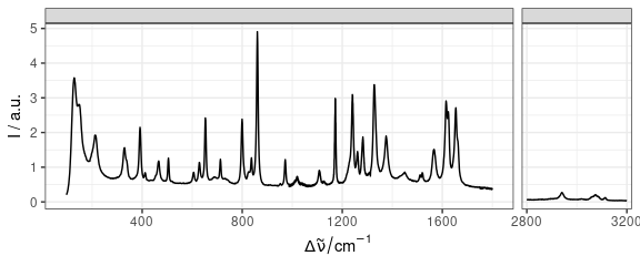
Figure 14: Plot separate regions of specra.
Session Info
Session info
sessioninfo::session_info("hyperSpec")
#> ─ Session info ───────────────────────────────────────────────────────────────────────────────────
#>  setting  value
#>  version  R version 4.3.0 (2023-04-21)
#>  os       Ubuntu 22.04.2 LTS
#>  system   x86_64, linux-gnu
#>  ui       X11
#>  language en
#>  collate  C.UTF-8
#>  ctype    C.UTF-8
#>  tz       UTC
#>  date     2023-04-23
#>  pandoc   2.19.2 @ /usr/bin/ (via rmarkdown)
#>
#> ─ Packages ───────────────────────────────────────────────────────────────────────────────────────
#>  package        * version      date (UTC) lib source
#>  brio             1.1.3        2021-11-30 [2] RSPM
#>  callr            3.7.3        2022-11-02 [2] RSPM
#>  cli              3.6.1        2023-03-23 [2] RSPM
#>  colorspace       2.1-0        2023-01-23 [2] RSPM
#>  crayon           1.5.2        2022-09-29 [2] RSPM
#>  deldir           1.0-6        2021-10-23 [2] RSPM
#>  desc             1.4.2        2022-09-08 [2] RSPM
#>  diffobj          0.3.5        2021-10-05 [2] RSPM
#>  digest           0.6.31       2022-12-11 [2] RSPM
#>  dplyr            1.1.2        2023-04-20 [2] RSPM
#>  ellipsis         0.3.2        2021-04-29 [2] RSPM
#>  evaluate         0.20         2023-01-17 [2] RSPM
#>  fansi            1.0.4        2023-01-22 [2] RSPM
#>  farver           2.1.1        2022-07-06 [2] RSPM
#>  fs               1.6.1        2023-02-06 [2] RSPM
#>  generics         0.1.3        2022-07-05 [2] RSPM
#>  ggplot2        * 3.4.2        2023-04-03 [2] RSPM
#>  glue             1.6.2        2022-02-24 [2] RSPM
#>  gtable           0.3.3        2023-03-21 [2] RSPM
#>  hyperSpec      * 0.200.0.9000 2023-04-23 [2] Custom
#>  hySpc.testthat   0.2.1        2020-06-24 [2] RSPM
#>  interp           1.1-4        2023-03-31 [2] RSPM
#>  isoband          0.2.7        2022-12-20 [2] RSPM
#>  jpeg             0.1-10       2022-11-29 [2] RSPM
#>  jsonlite         1.8.4        2022-12-06 [2] RSPM
#>  labeling         0.4.2        2020-10-20 [2] RSPM
#>  lattice        * 0.21-8       2023-04-05 [4] CRAN (R 4.3.0)
#>  latticeExtra     0.6-30       2022-07-04 [2] RSPM
#>  lazyeval         0.2.2        2019-03-15 [2] RSPM
#>  lifecycle        1.0.3        2022-10-07 [2] RSPM
#>  magrittr         2.0.3        2022-03-30 [2] RSPM
#>  MASS             7.3-58.4     2023-03-07 [4] CRAN (R 4.3.0)
#>  Matrix           1.5-4        2023-04-04 [4] CRAN (R 4.3.0)
#>  mgcv             1.8-42       2023-03-02 [4] CRAN (R 4.3.0)
#>  munsell          0.5.0        2018-06-12 [2] RSPM
#>  nlme             3.1-162      2023-01-31 [4] CRAN (R 4.3.0)
#>  pillar           1.9.0        2023-03-22 [2] RSPM
#>  pkgconfig        2.0.3        2019-09-22 [2] RSPM
#>  pkgload          1.3.2        2022-11-16 [2] RSPM
#>  png              0.1-8        2022-11-29 [2] RSPM
#>  praise           1.0.0        2015-08-11 [2] RSPM
#>  processx         3.8.1        2023-04-18 [2] RSPM
#>  ps               1.7.5        2023-04-18 [2] RSPM
#>  R6               2.5.1        2021-08-19 [2] RSPM
#>  RColorBrewer     1.1-3        2022-04-03 [2] RSPM
#>  Rcpp             1.0.10       2023-01-22 [2] RSPM
#>  RcppEigen        0.3.3.9.3    2022-11-05 [2] RSPM
#>  rematch2         2.1.2        2020-05-01 [2] RSPM
#>  rlang            1.1.0        2023-03-14 [2] RSPM
#>  rprojroot        2.0.3        2022-04-02 [2] RSPM
#>  scales           1.2.1        2022-08-20 [2] RSPM
#>  testthat         3.1.7        2023-03-12 [2] RSPM
#>  tibble           3.2.1        2023-03-20 [2] RSPM
#>  tidyselect       1.2.0        2022-10-10 [2] RSPM
#>  utf8             1.2.3        2023-01-31 [2] RSPM
#>  vctrs            0.6.2        2023-04-19 [2] RSPM
#>  viridisLite      0.4.1        2022-08-22 [2] RSPM
#>  waldo            0.4.0        2022-03-16 [2] RSPM
#>  withr            2.5.0        2022-03-03 [2] RSPM
#>  xml2             1.3.3        2021-11-30 [2] RSPM
#>
#>  [1] /tmp/Rtmp4dFdQI/temp_libpath151074fd346f
#>  [2] /home/runner/work/_temp/Library
#>  [3] /opt/R/4.3.0/lib/R/site-library
#>  [4] /opt/R/4.3.0/lib/R/library
#>
#> ──────────────────────────────────────────────────────────────────────────────────────────────────